Method 1: Lerp
The easiest way to smooth stuff is with lerp. I wrote about it here. It's really popular for games, especially in Unity. It's not a good method, but it's a nice intro to the topic.
The idea is you start at some value, then pick a target value. Each frame you move a little bit closer to the target by some percentage. The slower you move, the smoother your path becomes.
current = lerp(current, target, factor);Here's a demo with the smooth version in white. Click and drag to draw your own signal!
There's 3 big problems with this method, which all smoothing methods suffer from.
Problem 1: Phase shift
If you set the slider really low, it looks like the graph moves to the right. This is called phase shift.
It happens since the value is too lazy in moving to the target, so it sticks near the previous value and smears out the graph.
Phase shift is a popular topic in music, you'll find many audio engineers rambling about it online (Dan Worrall is my favourite). When you use an equalizer on music (for example to boost the bass), it usually adds a bit of phase shift. Some plugins (like Plugindoctor) even show you the exact phase shift you'll get. This is called the phase response.
Phase shift is a natural part of the universe so there's nothing wrong with it, but it's annoying if you want stuff to line up. The lazy way is shifting over the graph. The proper way is using linear phase filters. Linear phase filters always need values forwards in time as well as backwards.
The simplest way is smoothing forwards, then smoothing backwards. This cancels out the phase shift and makes a linear phase filter. Here's a demo with the original version in red, and the linear phase version in green.
Problem 2: Oversmoothing
You'll find this method is hard to control. It tends to smooth everything too much or not enough.
This is because of the order of the filter. The order basically means how sharp and precise a filter is. Here's a nice diagram from Electronics Tutorials. You can see as the order increases the curve gets steeper, meaning it cuts precisely and doesn't smudge everything.
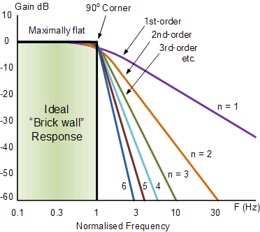
Lerp is a first order lowpass, so it's pretty blunt and tends to smudge everything out.
Turns out there's a cool trick to improve it. If you stack a bunch of low order filters, you approximate a high order filter. This works surprisingly well, though it's much slower and smudgier than doing it properly.
Here's a demo with the original filter in red, and the layered filters coloured towards purple. Try drawing some data and watch it move!
Problem 3: Undershooting
When the slider is below 1, it never actually reaches the target.
You can tell from the formula. Lerp does a weighted sum of two values, as I wrote here.
lerp(a, b, factor) = (1 - factor) * a + factor * bFor example if the factor is 0.9, it takes 10% of the current value and adds on 90% of the target value.
lerp(current, target, 0.9) = 0.1 * current + 0.9 * targetYou can't get 100% of the target value unless the factor is 1, which doesn't really count.
Here's a demo where the white line targets the red line. It always lies below the red line unless the factor is 1.
Running this in Houdini
To get this into Houdini, we need a way to access the previous frame. Luckily there's many ways to do this.
Option 1: Solver
Solvers are the most accurate and robust for this method. They run in sequence and never skip any frames, so if we had a huge jolt it continues smoothing out the impact forever. However they can't be run in parallel, so they're not ideal for farms.
First add a Solver node, then a Point Wrangle inside. Plug the the current animation (Input_1) into the second wrangle input.
Now we can write the formula in VEX. In solvers, @P is the current position. The second input we connected @opinput1_P is the latest animation, which is our target position.
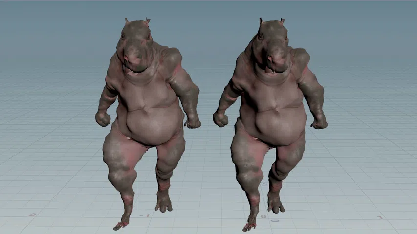
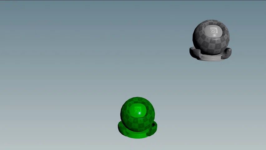
v@P = lerp(v@P, v@opinput1_P, chf("factor"));Here's before and after. It smooths out most of the noise, but reduces the range of motion too much.
Although solvers are ideal, we can get a decent approximation with Trail.
Option 2: Trail
Instead of sampling all past frames, it's faster to sample a handful of past frames and try to guess the future from them. This is called a sliding window technique, which Catherine used for her demo. It's good for production since it can be batch processed and run in parallel. However it's bad news for lerp, since lerp can't react to jolts if it doesn't know they happened.
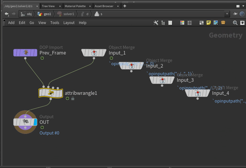
To try it anyway, add a Trail node and a Point Wrangle. Plug Trail into the second wrangle input.

For dense meshes, it helps to cache Trail for better performance.
Now we need to extract positions from different frames. This is done using point(). It has 3 arguments, but we only care about the last one.
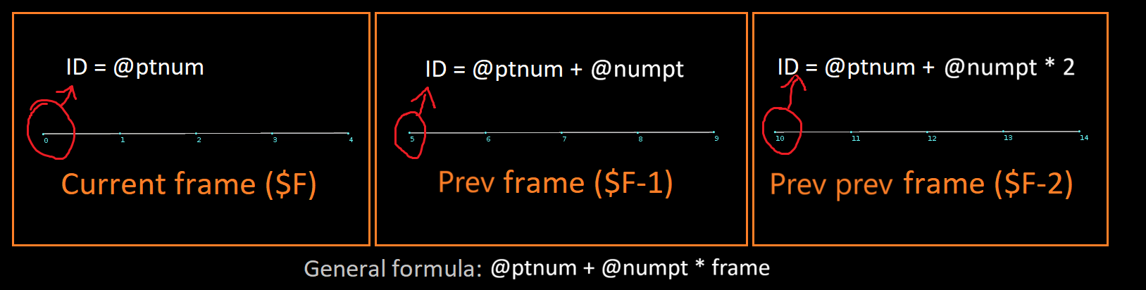
vector pos = point(0, "P", point_number);Given the current point number @ptnum, we need to find the matching point number on the previous frame. Assuming the topology stays the same, you'll find a pattern. Let's say your @ptnum is 0. If the mesh has 5 points, your @ptnum on the previous frame will be 5, 10, 15, 20 and so on. This happens since the Trail node merges batches of 5 points per frame.
Using i@numpt to get the number of points in the mesh, the general formula is @ptnum + i@numpt * frame
Using this idea we can lerp through the positions from past to present, just like with the solver. No dictionaries or maps required!
// Make sure this matches your trail node
int trail_length = chi("../trail1/length");
// Start at the last frame's position (the oldest frame)
v@P = point(1, "P", i@ptnum + i@numpt * (trail_length - 1));
// Lerp from the past to the present, like the solver except manually
for (int frame = 1; frame < trail_length; ++frame) {
// Get the corresponding point position on the next frame
vector target_pos = point(1, "P", i@ptnum + i@numpt * (trail_length - 1 - frame));
// The magic formula
v@P = lerp(v@P, target_pos, chf("factor"));
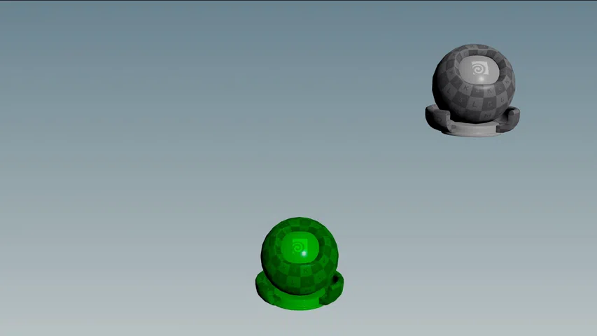
}Here's before and after. It looks pretty similar, but jitters more since it keeps forgetting past samples.
Sadly this version suffers from phase shift, just like the solver. The great thing with Trail is it doesn't have to. We can make linear phase filters and stack them too!
Linear phase version
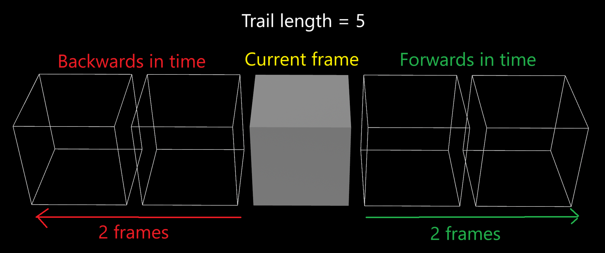
First we need a way to get frames forwards in time as well as backwards. This is as easy as adding a Time Shift node after Trail.
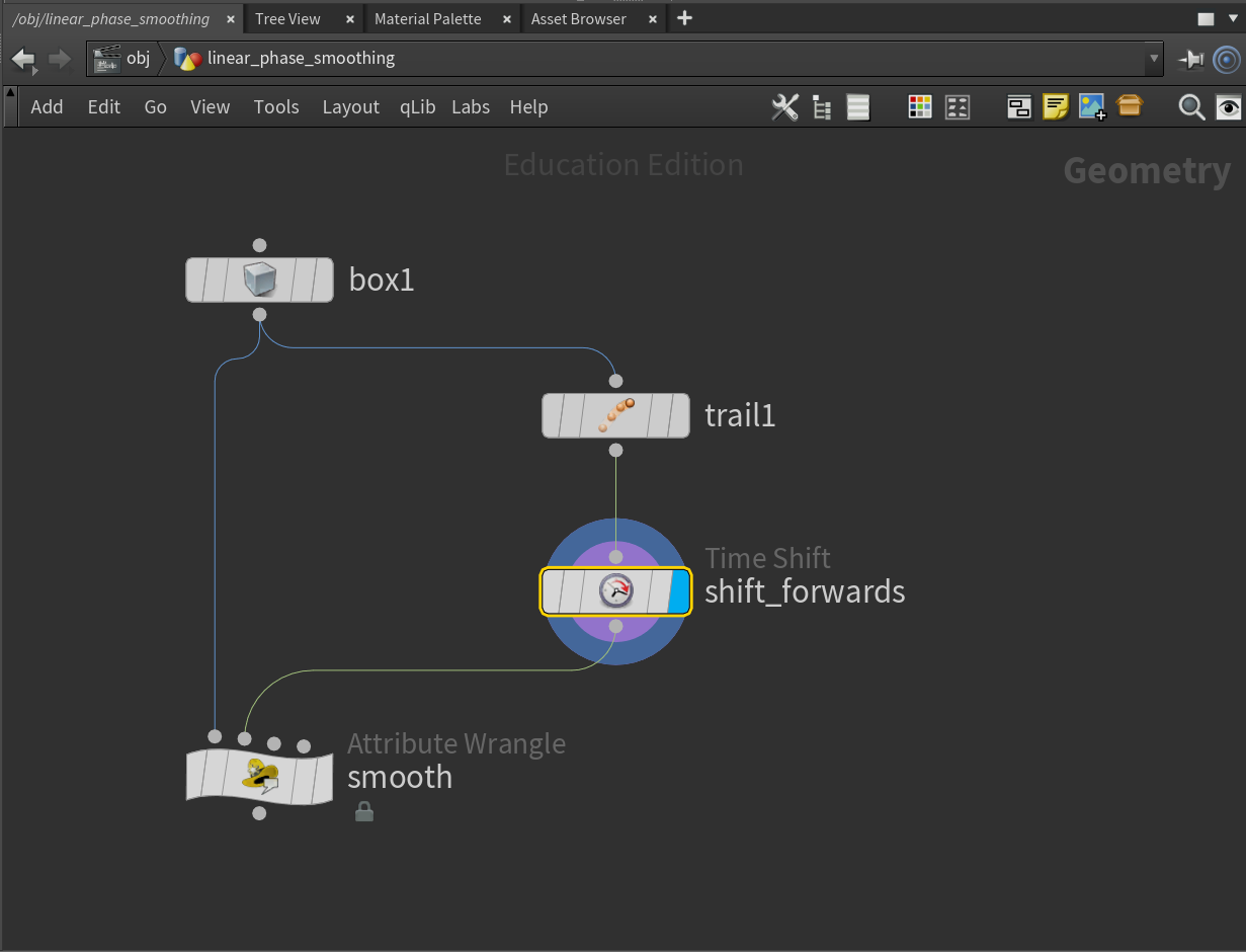
Set the frame offset to $F + (ch("../trail1/length") - 1) / 2. This centers the current frame, so we have the same number of frames forwards and backwards in time.
Next we can reuse the same frame offset idea from before, except this time filtering in both directions.
// Make sure this matches your trail node
int trail_length = chi("../trail1/length");
float factor = chf("factor");
int layers = chi("layers");
// Build an array of all positions on all frames
// For optimization, you could do a forward lerp in here
vector pos[];
resize(pos, trail_length);
for (int frame = 0; frame < trail_length; ++frame) {
pos[frame] = point(1, "P", i@ptnum + i@numpt * (trail_length - 1 - frame));
}
// Smooth a bunch of times in a row (if you want)
for (int i = 0; i < layers; ++i) {
// Smooth forwards in time
vector current_pos = pos[0];
for (int frame = 1; frame < trail_length; ++frame) {
// The magic formula
pos[frame] = lerp(current_pos, pos[frame], factor);
current_pos = pos[frame];
}
// Smooth backwards in time
current_pos = pos[trail_length - 1];
for (int frame = trail_length - 2; frame >= 0; --frame) {
// The magic formula
pos[frame] = lerp(current_pos, pos[frame], factor);
current_pos = pos[frame];
}
}
// Get the center frame, which is our frame
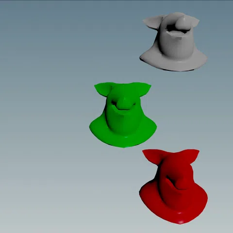
v@P = pos[trail_length / 2];Thanks to looking into the future, we can anticipate motion before it even happens. Here's a demo with the linear phase version in green and the original version in red.
While lerp works OK, there's plenty of fancier methods of smoothing out stuff. Let's learn about convolution!
Method 2: Convolution
Note Houdini's built-in Filter node works for convolution, but not with custom kernels! See Mark Fancher's tutorial.
Convolution solves many problems we were having before. It's linear phase and only needs a handful of frames, making it perfect for batch processing. It's a weighted sum just like lerp, but it's much more powerful than you'd expect. It works for smoothing, sharpening, embossing and all kinds of cool filters.
It works by picking a value, sampling the neighbours around it, multiplying them and adding them together. It's like what we did with lerp, except now we have precise control over how much each neighbour contributes to the final result. We can totally ignore neighbours or even flip their influence.
For example, say you want each value to be the average of its 2 neighbours. For that you can use the kernel [0.5, 0, 0.5].
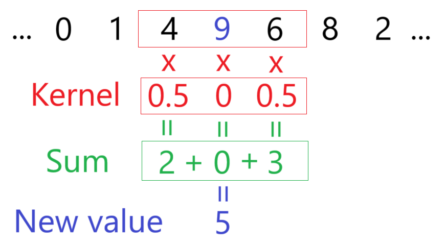
Here we sample 9's neighbours (4 and 6), then calculate 4 * 0.5 + 9 * 0 + 6 * 0.5 = 5. In other words, ignore 9 and average 4 and 6 together.
The key idea of convolution is you can slide the kernel up and down. Click and drag to see what I mean!
Tick "Convolve All" to see the full convolution, then mess with the weights to see what you find! Here's a few you can try:
- The kernel
[1, 0, 0]shifts everything 1 unit to the right. - The kernel
[0, 0, 1]shifts everything 1 unit to the left. - The kernel
[0, 1, 0]keeps everything the same. - The kernel
[1, 1, 1]sums all 3 values together. - The kernel
[1, 1, 0]sums the previous and current value. - The kernel
[0, 1, 1]sums the current and next value. - The kernel
[1, 0, 1]sums both neighbours. - The kernel
[0.5, 0, 0.5]averages the two neighbours together. - The kernel
[0.5, 0.5, 0]averages the previous and current value. - The kernel
[0, 0.5, 0.5]averages the current and next value.
With a tiny size 3 kernel, we can already do so many things. Hopefully this gives you an idea of how powerful and versatile convolution is.
Gaussian blur
Gaussian blur is one of the many things we can do with convolution. We just need to replace our kernel with a gaussian kernel. It looks like this.
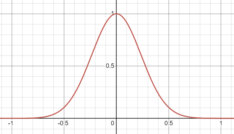
Stripping the formula to the bones, you can write it as exp(-x * x / (size * size)), where x is the value and size is the width of the shape. It extends infinitely, so you need to pick a size that fits most of it between -1 and 1. I found dividing size by 3 works pretty well, or in other words exp(-9 * x * x / (size * size)). Then we normalize it so all values add to 1.
And just like that we have gaussian blur! Change the kernel size to set the intensity.
Running this in Houdini
To get this into Houdini, we can reuse the trail setup from the lerp section with a few minor changes.
First we need to make the kernel. We can do it in a Detail Wrangle since it never changes and only needs to be built once.
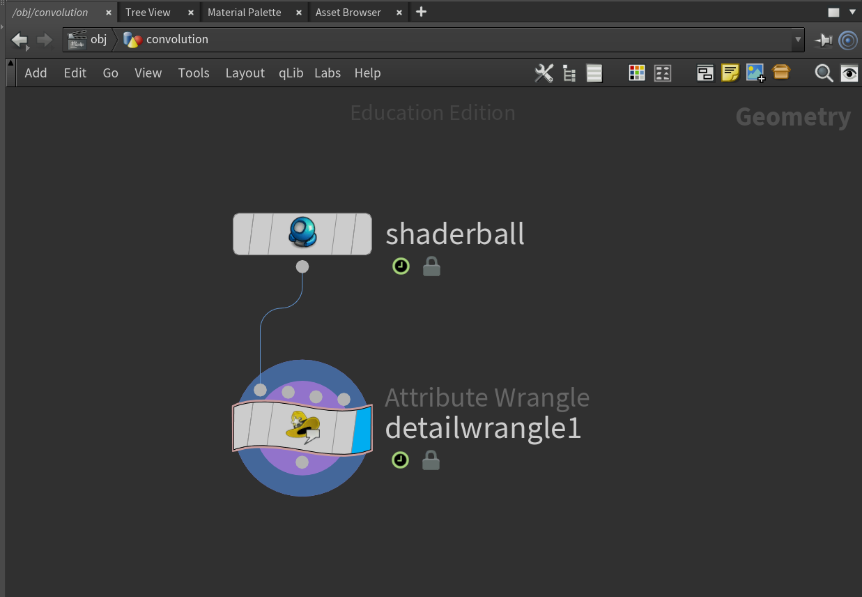
Let's store the kernel in a detail attribute. The syntax is pretty ugly, f[]@kernel just means an array of floats.
// Make sure this matches your trail node
int trail_length = chi("../trail1/length");

// Width of shape, divided by 3 so it fits snugly between -1 and 1
float size = trail_length / 3.0;

// Preallocate array size
resize(f[]@kernel, trail_length);
f@kernel_sum = 0;

// Build gaussian kernel (array of floats)
for (int i = 0; i < trail_length; ++i) {
	// Center it on the middle value
	float x = i - (trail_length - 1) / 2.0;
	f[]@kernel[i] = exp(-x * x / (size * size));
	f@kernel_sum += f[]@kernel[i];
}
Now we dump in the Trail, Time Shift and Point Wrangle from the lerp section. Like before, the frame offset is $F + (ch("../trail1/length") - 1) / 2.
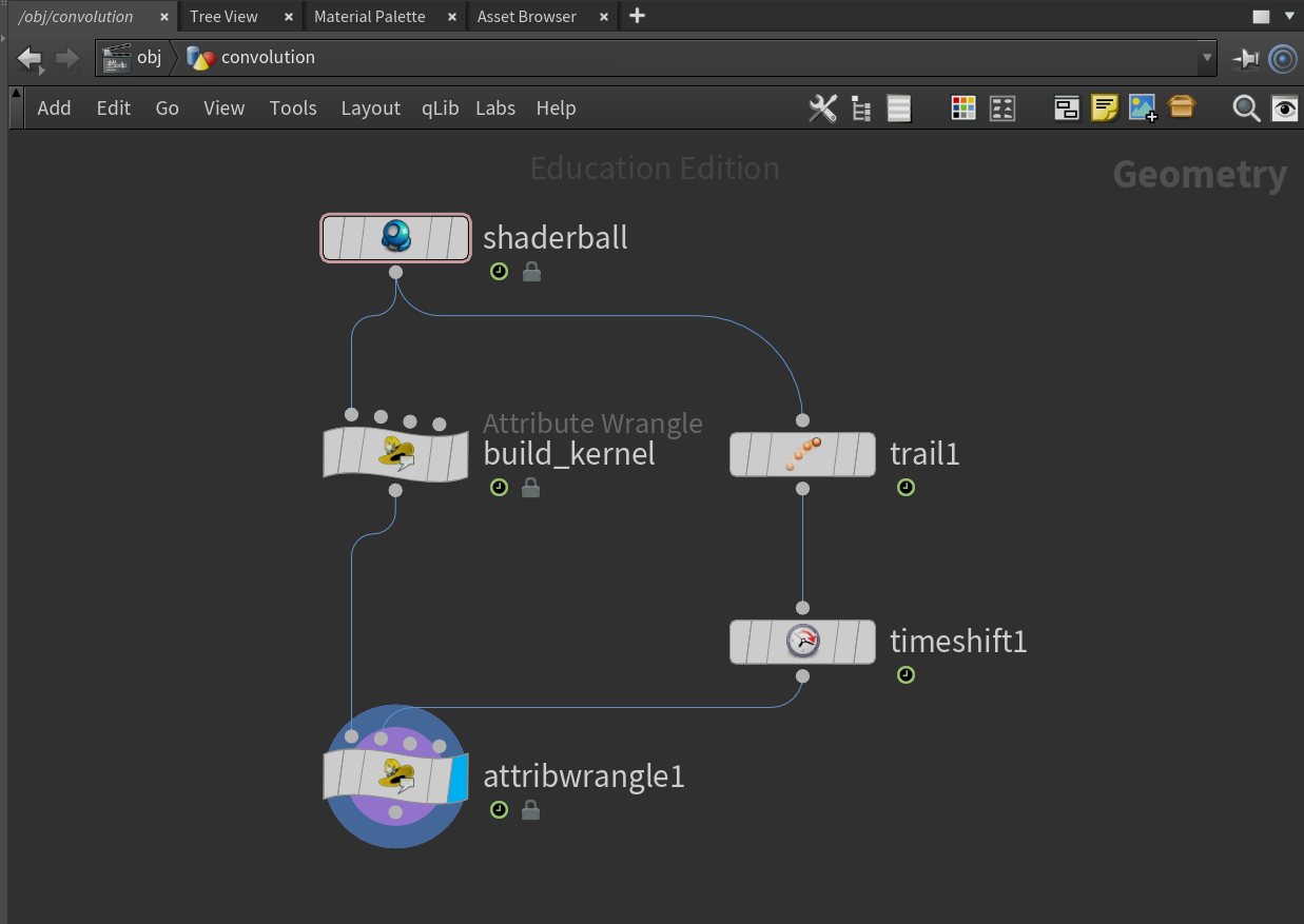
Now onto the convolution. It's surprisingly easy since Trail and Time Shift did the hard work for us. We just need to add up all the values multiplied by their respective weights.
// Make sure this matches your trail node
int trail_length = chi("../trail1/length");

// Convolve all frames to get the current frame
vector pos_total = 0;
for (int frame = 0; frame < trail_length; ++frame) {
	vector pos = point(1, "P", i@ptnum + i@numpt * (trail_length - 1 - frame));
	pos_total += pos * f[]@kernel[frame];
}

// Normalize so it adds to 1
v@P = pos_total / f@kernel_sum;
The trail length directly controls the amount of blur. The more frames we sample, the more we can blur.
| 23 frames | 61 frames |
|---|---|
|
|
Now I know what you're thinking. This looks exactly like lerp from before! What's the point of going through all that effort?
Well firstly, it actually reaches the target unlike lerp. And secondly, you can swap out the kernel to get cool effects!
Cool kernels
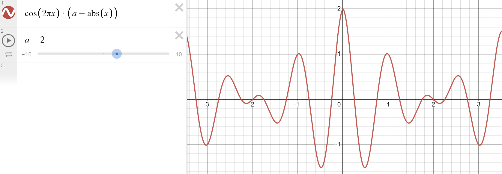
Here's a cool kernel I made by accident. It turns any animation into an incredible springy mess!
// Make sure this matches your trail node
int trail_length = chi("../trail1/length");

// Preallocate array size
resize(f[]@kernel, trail_length);
f@kernel_sum = 0;

// Build insane kernel
float insanity = 2;
for (int i = 0; i < trail_length; ++i) {
	// Center it on the middle value
	float x = i - (trail_length - 1) / 2.0;
	// Normalize the range
	x /= trail_length;
	// Invoke madness
	f[]@kernel[i] = cos(2 * PI * x) * (insanity - abs(x));
	f@kernel_sum += f[]@kernel[i];
}
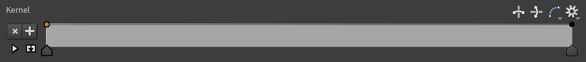
Drawing kernels with ramps
This way of building kernels is ugly and hard. It'd be nicer if we could draw kernels visually with a ramp.
For that we can delete the Detail Wrangle and use a single Point Wrangle, since the ramp stores the kernel for us.
// Make sure this matches your trail node
int trail_length = chi("../trail1/length");

// Convolve all frames to get the current frame
vector pos_total = 0;
float kernel_sum = 0;

for (int frame = 0; frame < trail_length; ++frame) {
	vector pos = point(1, "P", i@ptnum + i@numpt * (trail_length - 1 - frame));
	float weight = chramp("kernel", float(frame) / (trail_length - 1));
	pos_total += pos * weight;
	kernel_sum += weight;
}

// Normalize so it adds to 1
if (chi("normalize_kernel")) {
	pos_total /= kernel_sum;
}

v@P = pos_total;
Now we can easily experiment with different shapes! I found this one also has a crazy effect on the motion.
TODO: ADD DEMO AND HIP FILE
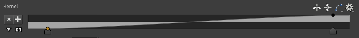
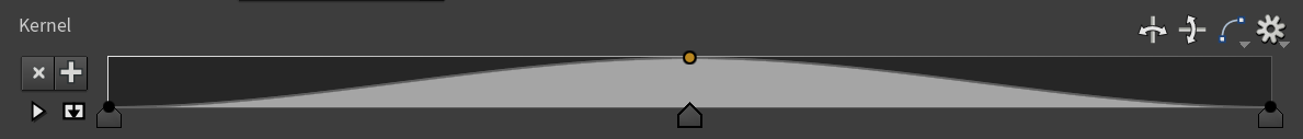
Sharpening kernels
Sharpening kernels are usually positive in the middle and negative on the sides. Here's one I drew to exaggerate the motion.
| 15 frames | 35 frames |
|---|---|
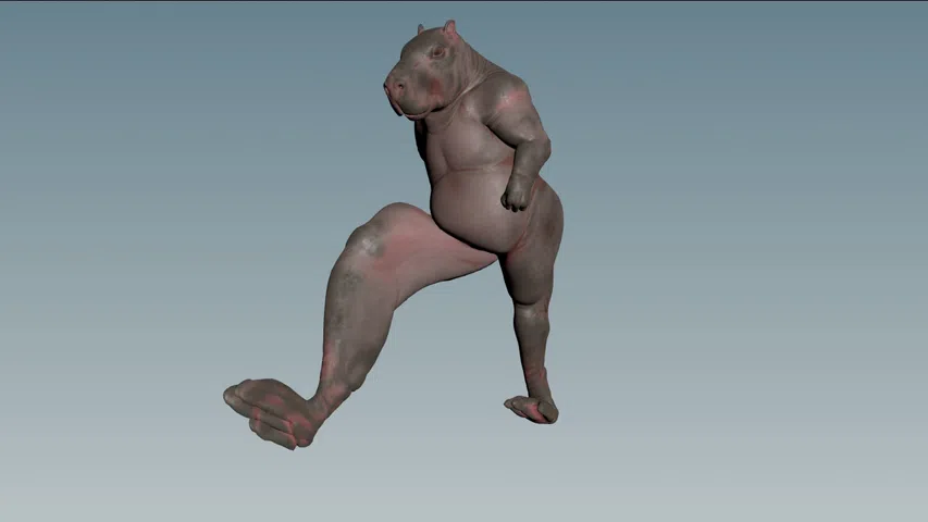
|
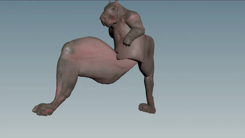
|
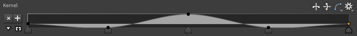
Blurring kernels
We can make blurry kernels too, just like before. To make box blur (also called a moving average), just draw a flat line.
To approximate gaussian blur, draw a bell curve centered at 0.5.
Here's a demo with gaussian blur in blue and box blur in green. Box blur tends to blur more aggressively since it uses all samples equally.
Topology convolution
Going off track for a bit, I started wondering what happens if you convolve geometry instead of time.
Convolution just needs neighbours and weights. Let's sample a bunch of nearby points, multiply them by weights and add them together. Just like Attribute Blur, we could do it by connectivity or proximity.
Option 1: Connectivity
If the geometry is connected by edges, the neighbors for any point are found by travelling along the edges. Now we have neighbors, we just need weights. Let's weigh each point based on how many edges away it is.
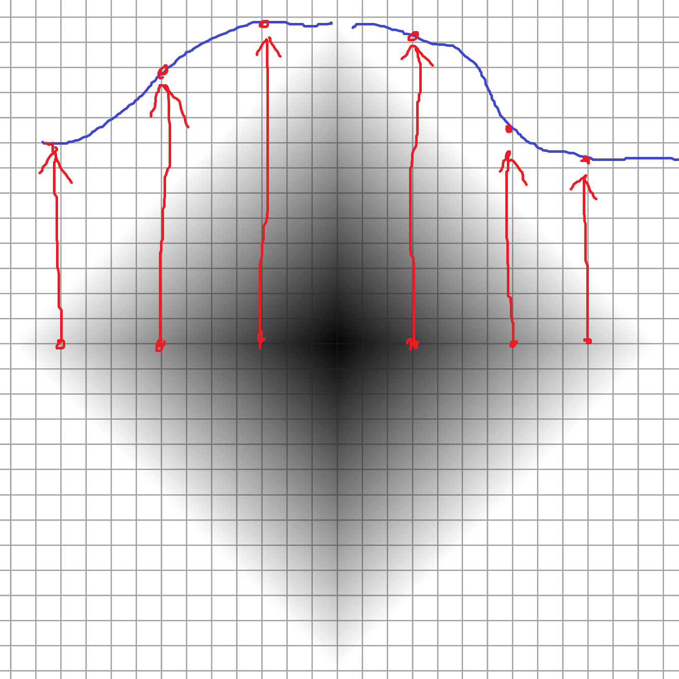
Below I picked the red point as the center, then used Group Expand to generate a step attribute. The step attribute is how many edges away each point is. You can see the nearby points are darker, and the further ones are brighter.
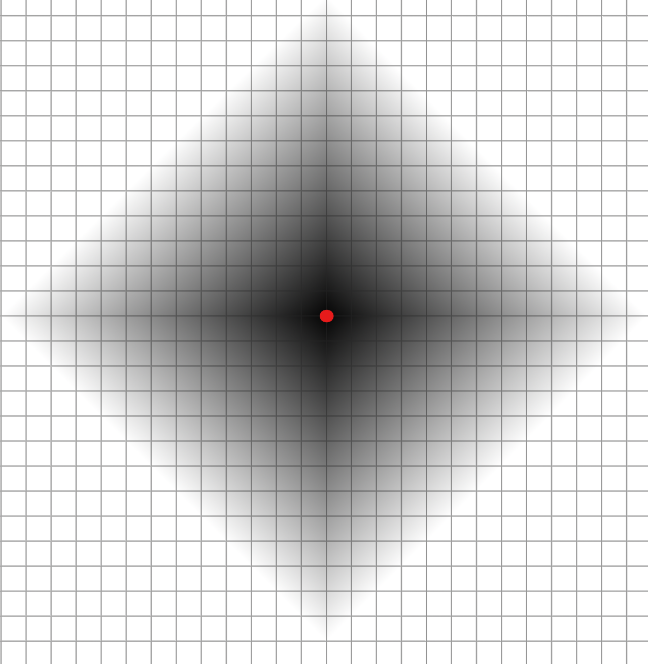
Now let's remap the step attribute to a new value using a ramp. This ramp is our convolution kernel.
Sadly I couldn't find an easy way to define up, down, left and right. Instead I cut the ramp in half and mapped all directions equivalently.
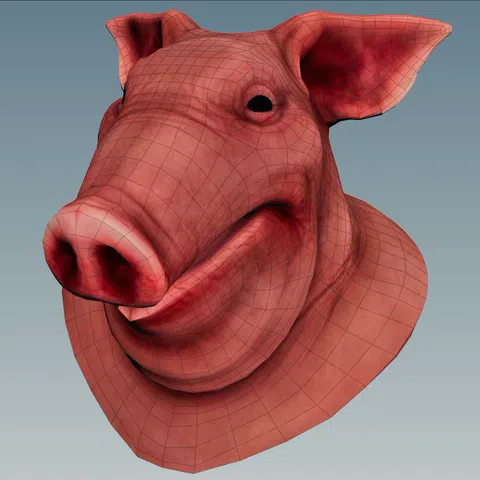
In 3D this makes a bulge symmetrical in all directions away from the center point.
Now we sum the results, and repeat this for all points. I originally did this by remaking Group Expand in VEX, which is very slow.
int visited_points[] = array(i@ptnum);
int last_points[] = visited_points;
// Sum the current point immediately
float kernel_sum = chramp("kernel", 0);
vector pos_total = point(0, "P", i@ptnum);
pos_total *= kernel_sum;
// Convolve based on neighbouring points, like Group Expand
// Adapted from https://www.sidefx.com/forum/topic/77827
int depth = chi("depth");
for (int i = 1; i <= depth; ++i) {
int new_points[];
foreach (int pt; last_points) {
// Find all points connected to the current one
int connected[] = neighbours(0, pt);
foreach (int c; connected) {
// find() is really slow, wish VEX had hashsets
// I tried dictionaries, they're even slower
if (find(visited_points, c) < 0) {
append(visited_points, c);
append(new_points, c);
// Sample kernel based on how many points away we travelled
// This is biased by density, ideally scale it by edge length travelled
vector pos = point(0, "P", c);
float weight = chramp("kernel", float(i) / depth);
kernel_sum += weight;
pos_total += pos * weight;
}
}
}
last_points = new_points;
}
// Normalize so it adds to 1
if (chi("normalize_kernel")) {
pos_total /= kernel_sum;
}
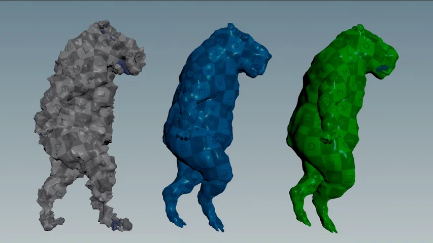
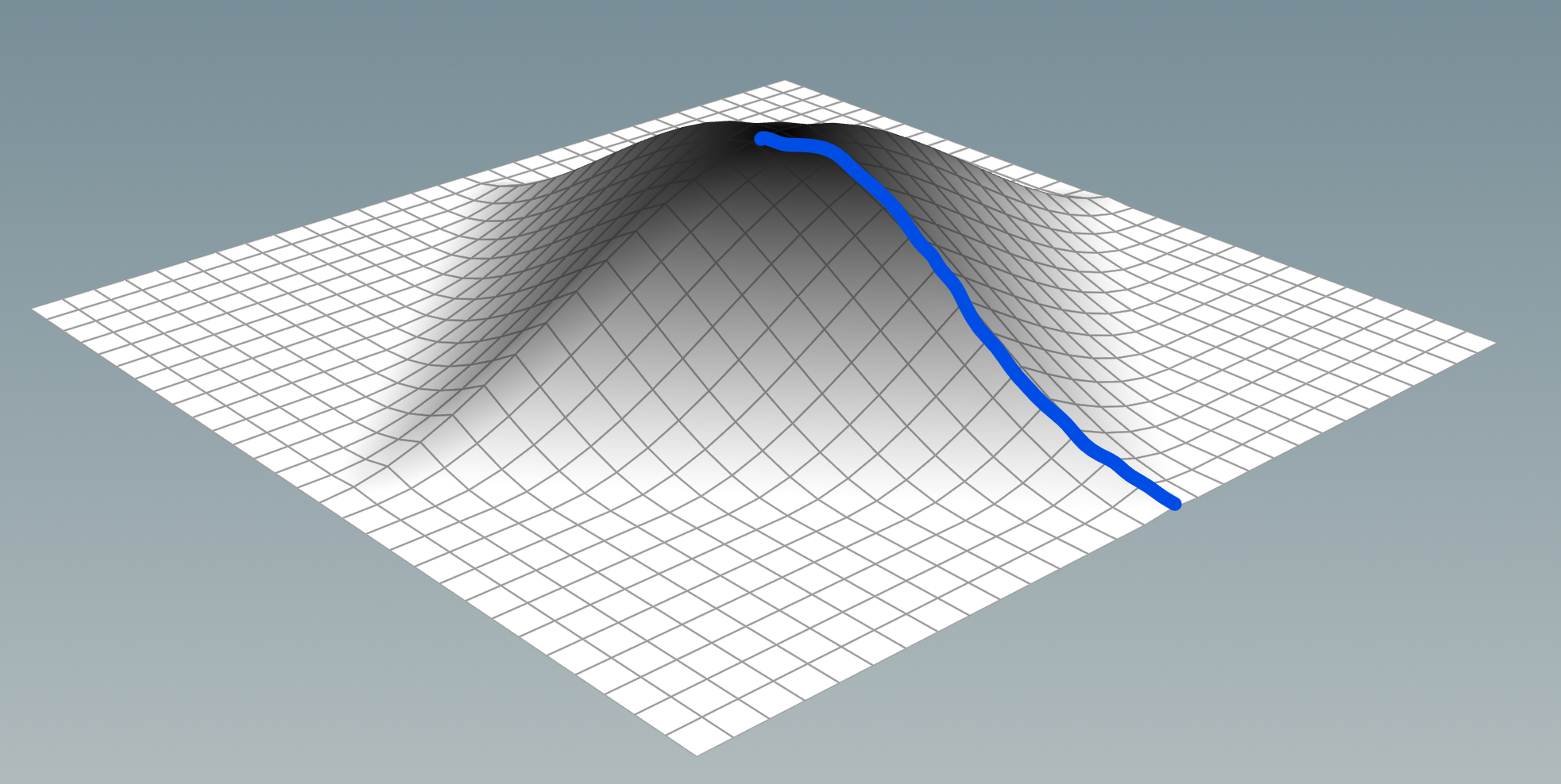
v@P = pos_total;Here's a demo using a gaussian kernel. The features get smoothed by different amounts since I didn't consider edge lengths.

A much faster method is using Group Expand or Edge Transport in a For-Each Point loop. It's hard to explain here, so I included both methods in the HIP file.
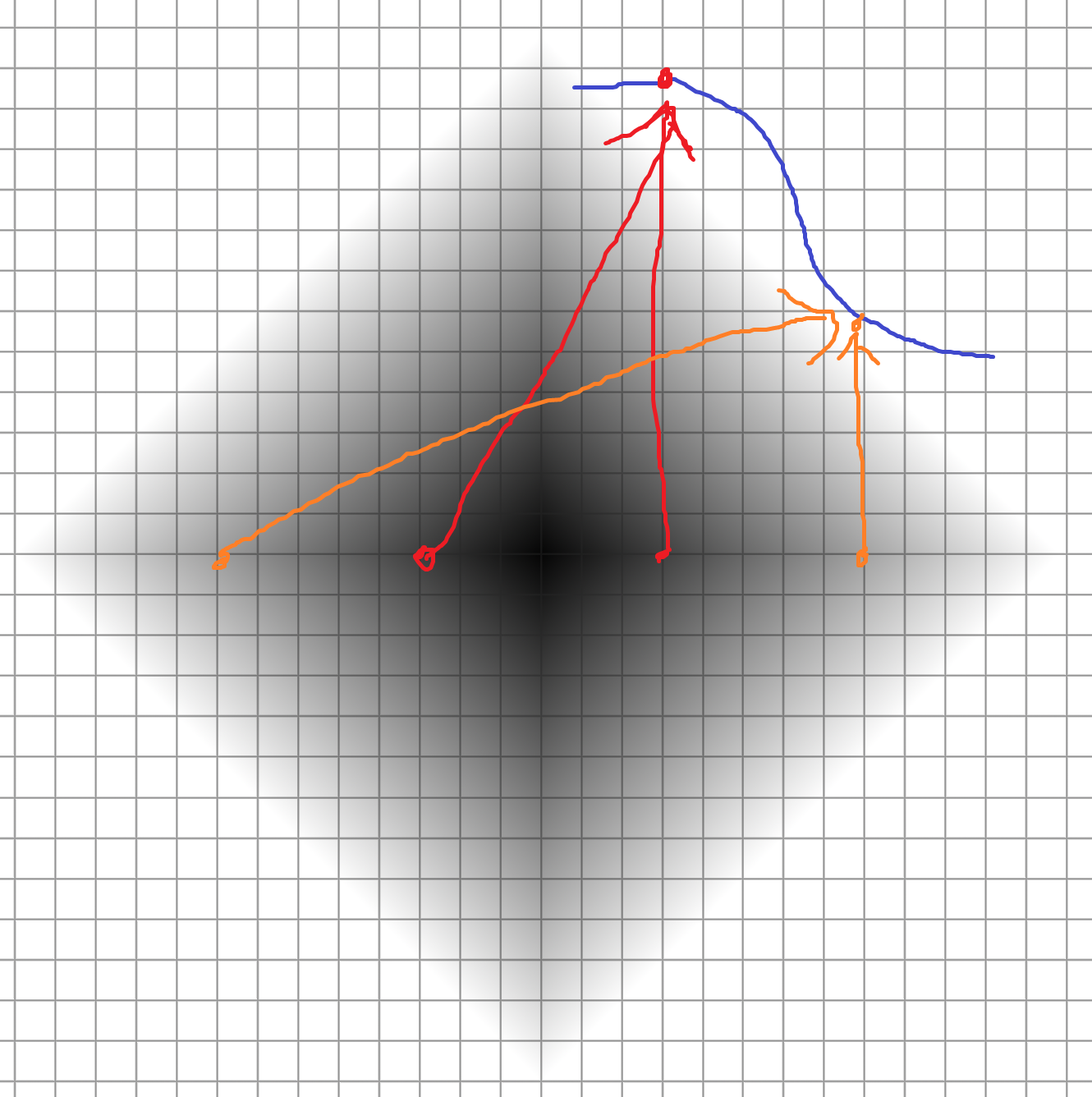
Group Expand is identical to the VEX method, while Edge Transport sums the edge lengths. By considering edge lengths you can see the smoothing is evenly distributed across the entire geometry, reducing the distortion of the features.
Option 2: Proximity
If we have a disconnected point cloud, we can sample neighbors in a sphere and weigh them by their distance to the center.
I thought it'd work better since edge lengths don't matter, but it still gets biased by point clusters similar distances away.
// Clamp to prevent 0 distance
float max_dist = max(1e-8, chf("max_distance"));
int points[] = pcfind(0, "P", v@P, max_dist, i@numpt);

vector pos_total = 0;
float kernel_sum = 0;

// Sample kernel based on how far away each point is
foreach (int pt; points) {
	vector pos = point(0, "P", pt);
	float dist = distance(pos, v@P);
	float weight = chramp("kernel", dist / max_dist);
	pos_total += pos * weight;
	kernel_sum += weight;
}

// Normalize so it adds to 1
if (chi("normalize_kernel")) {
	pos_total /= kernel_sum;
}

v@P = pos_total;
This looks similar to Edge Transport, which makes sense since both are distance-based methods.
Anyway, back on track. Let's jump to lerp's big brother, biquad filters!
Method 3: IIR filters
Biquad filters are super popular for music and sound design. They're used for most digital EQs, so when you boost the bass or cut the treble, you're probably using a biquad filter. They give full control over the frequency response with very little effort.
Have a play with the demo below. Try to get a feel for how time and frequency interact.
Time Domain
Frequency Domain
Here's some ideas you can try:
- A lowpass filter dampens high frequencies. Try to dampen the noise without affecting the main sine wave.
- A highpass filter dampens low frequencies. Try to dampen the main sine wave without affecting the noise.
- A bandpass filter isolates a certain frequency. Try to isolate the main sine wave to cut the noise.
- A notch filter cuts out a certain frequency. Try to cut the main sine wave and identify its frequency.
- A peaking filter exaggerates or dampens a certain frequency. Try to exaggerate the main sine wave.
- A low shelf filter exaggerates or dampens low frequencies. Try to dampen the main sine wave.
- A high shelf filter exaggerates or dampens high frequencies. Try to exaggerate the noise.
- Butterworth filters are steeper, made by stacking biquads with certain settings. Try to isolate the main sine wave.
The big picture
So how do biquad filters work? Originally I had no clue. There's a famous resource on them, Robert Bristow-Johnson audio EQ cookbook. It has a beautiful C version by Tom St Denis, which I blindly copy pasted like everyone else.
Now I have a better idea of the big picture, so here's what I know.
IIR vs FIR filters
Here's the truth, I've been lying to you. I left out a key detail until now.
There's 2 main types of filters: IIR and FIR. Surprise! Lerp is an IIR filter, convolution is an FIR filter.
IIR filters
IIR stands for Infinite Impulse Response. This means the filter is recursive, and never settles to 0.
Lerp is a perfect example. It's recursive since it uses the previous output of itself, and always undershoots 0.
current = lerp(current, target, factor);Here's a demo with the impulse in white, and the impulse response in red. It goes forever!
FIR filters
FIR stands for Finite Impulse Response. This means the filter isn't recursive, and settles to 0 within a number of samples.
Convolution is a perfect example. Since the kernel has a fixed size, the response never extends beyond that range.
Here's a demo with a gaussian kernel. See how the shapes match? With convolution, the kernel IS the impulse response!
Because of this, we can turn any IIR filter into a FIR filter just by using the IIR impulse response as a kernel! I'll get into that later.
Lerp vs biquad filters
Lerp and biquad filters have lots in common. Both are IIR filters! To prove it, let's transform lerp into a biquad filter!
Let's start with the basic lerp code from before.
current = lerp(current, target, factor);Since it's recursive it runs every frame. It's a bit unclear how it'd run sequentially. Let's make it more obvious.
Say we have an input array x. We want to filter it and store the output in an array y. The current array index is n.
y[n] = lerp(y[n-1], x[n], factor);Now it clearly involves 2 things: the latest input x[n], and the previous filter output y[n-1].
In filter lingo, x[n] is called a feedforward coefficient, and y[n-1] is called a feedback coefficient.
Now I'll replace lerp with the math it uses internally.
y[n] = factor * x[n] + (1 - factor) * y[n-1];You can see it's a weighted sum of 2 values. Let's call the weights b0 and a1.
a1 = 1 - factor;
b0 = factor;
y[n] = b0 * x[n] + a1 * y[n-1];
Why am I doing all this boring stuff? To show you how it compares to a biquad filter!
Here's the Direct Form 1 biquad formula from the famous RBJ cookbook:
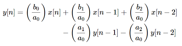
Currently we're missing a few coefficients. We've got b0 and a1, but we're missing a0, a2, b1 and b2.
In filter lingo, that means we've got a first order lowpass (single pole).
Biquad filters are second order, so they require 2 feedforward and 2 feedback coefficients.
TODO: FINISH THIS
Running this in Houdini
TODO: FINISH THIS
In the code above, you'll see variables called a0, a1, a2, a3 and a4. These are the coefficients of the filter.
Each filter type has different coefficients, so the first step is calculating them for the filter we want. Start by adding a Detail Wrangle.

Now let's steal the C code and translate it into VEX! One day I'll understand the math, but sadly not today.
// How many samples we're getting every second
float sample_rate = chf("sample_rate");

// Filter type: lowpass, highpass, bandpass, notch, peaking, low shelf or high shelf
int filter_type = chi("filter_type");

// Frequency of the filter, must be less than half the sample rate (Nyquist)
float freq = chf("frequency");

// Shape of the filter, used by all except low and high shelf filters
float Q = chf("Q");

// Gain in decibels, used by peaking, low shelf and high shelf filters
float db_gain = chf("gain_db");

// Shared between most filter types
float A = pow(10.0, db_gain / 40.0);
float w = 2.0 * PI * freq / sample_rate;
float sn = sin(w);
float cs = cos(w);
float alpha = sn / (2.0 * Q);
float beta = sqrt(A + A);

// Calculate the coefficients for each filter type
float a0, a1, a2, b0, b1, b2;
if (filter_type == 0) {
	// Low pass
	b0 = (1.0 - cs) / 2.0;
	b1 = 1.0 - cs;
	b2 = b0;
	a0 = 1.0 + alpha;
	a1 = -2.0 * cs;
	a2 = 1.0 - alpha;
} else if (filter_type == 1) {
	// High pass
	b0 = (1.0 + cs) / 2.0;
	b1 = -(1.0 + cs);
	b2 = b0;
	a0 = 1.0 + alpha;
	a1 = -2.0 * cs;
	a2 = 1.0 - alpha;
} else if (filter_type == 2) {
	// Band pass
	b0 = alpha;
	b1 = 0.0;
	b2 = -alpha;
	a0 = 1.0 + alpha;
	a1 = -2.0 * cs;
	a2 = 1.0 - alpha;
} else if (filter_type == 3) {
	// Notch
	b0 = 1.0;
	b1 = -2.0 * cs;
	b2 = 1.0;
	a0 = 1.0 + alpha;
	a1 = b1;
	a2 = 1.0 - alpha;
} else if (filter_type == 4) {
	// Peaking
	b0 = 1.0 + (alpha * A);
	b1 = -2.0 * cs;
	b2 = 1.0 - (alpha * A);
	a0 = 1.0 + (alpha / A);
	a1 = b1;
	a2 = 1.0 - (alpha / A);
} else if (filter_type == 5) {
	// Low shelf
	b0 = A * ((A + 1.0) - (A - 1.0) * cs + beta * sn);
	b1 = 2.0 * A * ((A - 1.0) - (A + 1.0) * cs);
	b2 = A * ((A + 1.0) - (A - 1.0) * cs - beta * sn);
	a0 = (A + 1.0) + (A - 1.0) * cs + beta * sn;
	a1 = -2.0 * ((A - 1.0) + (A + 1.0) * cs);
	a2 = (A + 1.0) + (A - 1.0) * cs - beta * sn;
} else if (filter_type == 6) {
	// High shelf
	b0 = A * ((A + 1.0) + (A - 1.0) * cs + beta * sn);
	b1 = -2.0 * A * ((A - 1.0) + (A + 1.0) * cs);
	b2 = A * ((A + 1.0) + (A - 1.0) * cs - beta * sn);
	a0 = (A + 1.0) - (A - 1.0) * cs + beta * sn;
	a1 = 2.0 * ((A - 1.0) - (A + 1.0) * cs);
	a2 = (A + 1.0) - (A - 1.0) * cs - beta * sn;
} else if (filter_type == 7) {
	// All pass (from https://webaudio.github.io/web-audio-api/#BiquadFilterNode)
	b0 = 1.0 - alpha;
	b1 = -2.0 * cs;
	b2 = 1.0 + alpha;
	a0 = b2;
	a1 = b1;
	a2 = b0;
}

// Final coefficients, these actually get used for filtering
f@a0 = b0 / a0;
f@a1 = b1 / a0;
f@a2 = b2 / a0;
f@a3 = a1 / a0;
f@a4 = a2 / a0;
This spits out the coefficients we need as detail attributes called @a0, @a1, @a2, @a3 and @a4. Brilliant!
Now we need to set the initial values of the filter, @x1, @x2, @y1 and @y2. Do this in a Point Wrangle after the Detail Wrangle.
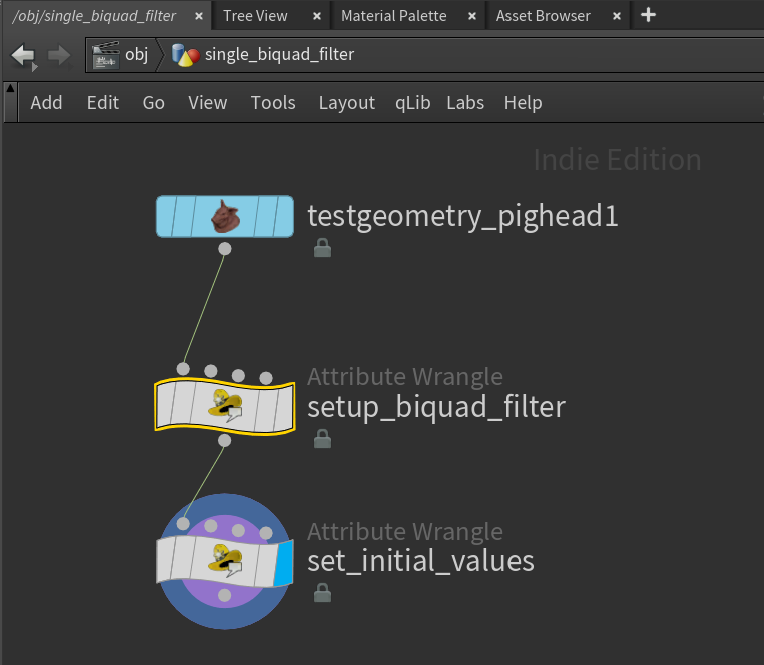
Since we haven't filtered anything yet, we can set the initial values to 0.
v@x1 = v@x2 = v@y1 = v@y2 = 0;Or if you really want, you can set them to the current position.
v@x1 = v@x2 = v@y1 = v@y2 = v@P;This helps the filter converge faster towards the target value. It's good for some filters like a lowpass, where the filtered value is similar to the original value. For others like a highpass, it makes it harder since it's further to travel.
Finally we can run the biquad filter using a Solver. Add a Solver node after the Point Wrangle.
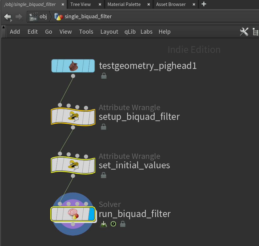
In the Solver, add a Point Wrangle with the current animation (Input_1) plugged into the second wrangle input.
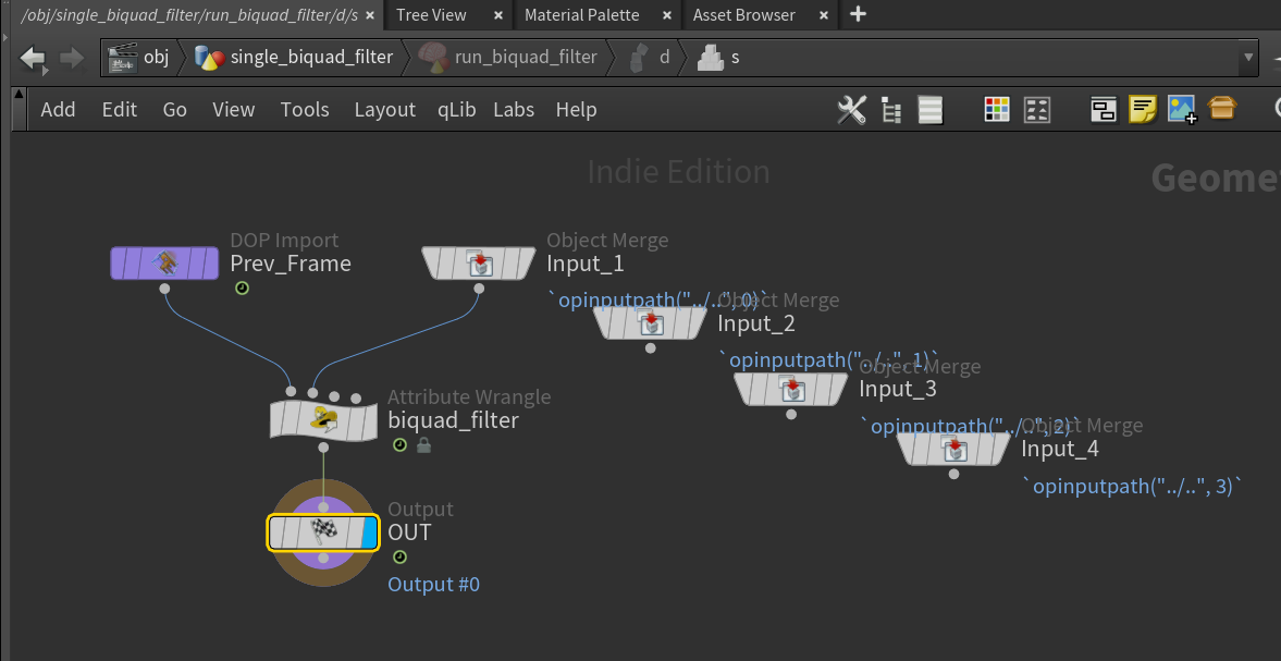
In the Point Wrangle is the heart of the filter. Just as before, it's only a few lines of code!
// Get current sample
vector sample = v@opinput1_P;

// Apply filter based on current sample
v@P = f@a0 * sample
    + f@a1 * v@x1
    + f@a2 * v@x2
    - f@a3 * v@y1
    - f@a4 * v@y2;

// Shift x1 to x2, sample to x1
v@x2 = v@x1;
v@x1 = sample;

// Shift y1 to y2, result to y1
v@y2 = v@y1;
v@y1 = v@P;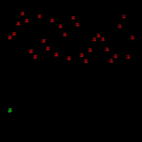
Oversampling
A popular music technique is oversampling, adding more detail to your signal. It helps biquad filters cramp less.
Sampled signals have limits in what they can store. One of these limits is the Nyquist frequency. It means anything above half the sample rate can't be stored with perfect quality. For example if your FPS is 24 Hz, you can only view sine waves up to 12 Hz. Anything faster appears to slow down, since the camera records slower than the object moves. This is known as aliasing.
This happens a lot in Houdini, like with motion blur of fast moving objects. If something moves at sonic speed, you need tons of substeps to accurately capture the movement.
Nyquist limits also apply to biquad filters. You can't make the frequency of a biquad filter higher than half the sample rate. It's impossible for sine waves above Nyquist to exist, so there's no point trying to filter them out.
Just like with motion blur, the solution is oversampling. In Houdini that means increasing the substeps on your Solver. If you double the substeps from 1 to 2, you're doubling the sample rate from 24 to 48. Now you can filter anything up to 24 Hz!
When setting up biquad coefficients, make sure your sample rate includes the substeps too!
Sample Rate = $FPS * ch("../solver/substep")Stacking filters
TODO: FINISH THIS
Method 4: FIR filters
Note Houdini's built-in Pass Filter node works for FIR filters!
FIR filters are the perfect marriage of convolution and biquad filters. It's convolution with the most powerful kernel in the world!
To understand them, let's go back to lerp. Remember how I said lerp is an IIR lowpass? What does IIR even mean?
IIR stands for Infinite Impulse Response. This means the filter runs forever, and you keep feeding it samples infinitely. This is great for intense smoothing, since it gives plenty of time to move towards the target value. But most of the time we don't have infinite samples, like with Trail we only get a few samples at a time!
You can't just chop a signal up, lerp each piece and expect good results.
The same thing happens when you use Trail with lerp. It adds more lumps and bumps instead of smoothing them out. If only there was a cleaner way to smooth pieces of a signal. Turns out there is, FIR filters!
FIR stands for Finite Impulse Response. This means the signal and filter have a fixed size, just like Trail.
TODO: FINISH THIS
Further Reading
- 2nd Order Biquads (Robert Bristow-Johnson)
- 2nd Order Biquads in C (Tom St Denis)
- 1st Order Biquads (Robert Bristow-Johnson)
- Biquad Frequency Response Derivation (Robert Bristow-Johnson)
- Biquad Frequency Response Demo (ErBird)
- 1st/2nd Order Biquad Calculator (Nigel Redmon)
- Butterworth Q Calculator (Nigel Redmon)
- Pole-Zero Placement (Nigel Redmon)
- Digital Signals Theory (Brian McFee)
- Simple DFT in C++ (QuantitativeBytes)
- Fourier Transform Intro (3Blue1Brown)
- Fourier Transform Demo (Jez Swanson)