Houdini-Fun
CGWiki DLC
Various Houdini tips and tricks I use a bunch. Hope someone finds this helpful!
Rabbit Hole
These articles grew too long to fit here. They’re the most interesting in my opinion, so be sure to check them out!
- Vertex Block Descent in Houdini
- 3D Signed Distance Functions
- Lerp and Fit
- Waveforms
- Easings
- Normalized Device Coordinates
- 4D Geometry
- Time Smoothing (WIP, interactive!)
- Vexember 2023 (WIP)
- Sound Effects (WIP)
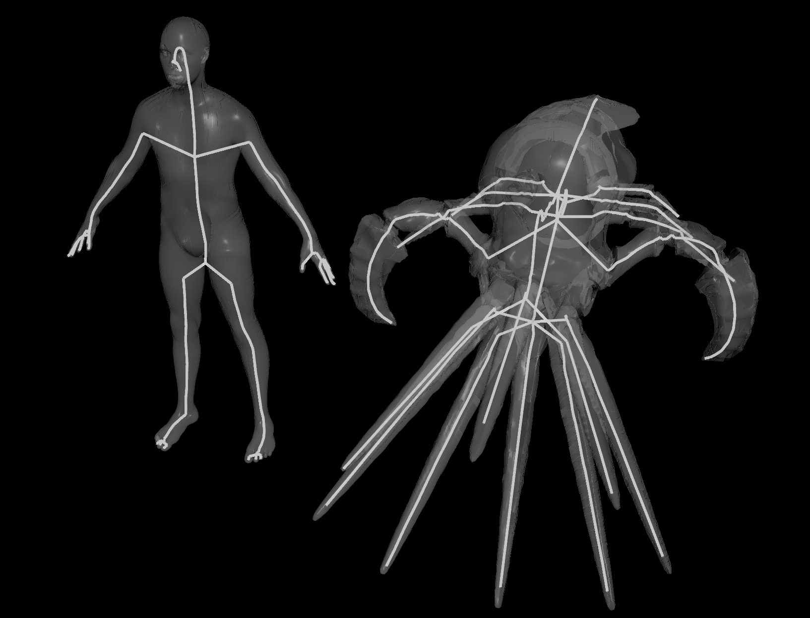
 HDA: Fast Straight Skeleton 3D
They added a new Laplacian node to Houdini 20.5. You can do cool frequency-based tricks with it.
One example is calculating a straight skeleton. You can do this with a Laplacian node followed by a Linear Solver set to “SymEigsShiftSolver”. This gives you a bunch of Laplacian eigenvectors, which are like frequencies making up a mesh.
The second lowest frequency (or eigenvector) is called the Fiedler vector. It follows the general flow of the geometry, which is great for straight skeletons. Also it’s orders of magnitude faster than Labs Straight Skeleton 3D!
Thanks to White Dog for letting me share this and suggesting improvements! It’s based on his Curve Skeleton example.
| Download the HDA! | Download the HIP file! | | — | — |
HDA: Rigid Piece Preroll
Most preroll nodes use position difference only. This is fine for translation but not rotation.
Extract Transform can be used to estimate the rotation difference too. This gives preroll for both rotation and translation.
This HDA works on single and multiple pieces, either packed or unpacked. For packed pieces, it uses their intrinsic transforms.
| Download the HDA! | Download the HIP file! | | — | — |
Simple spring solver
Need to overshoot an animation or smooth it over time to reduce bumps? Introducing the simple spring solver!

Recursive Version
I stole this from an article on 2D wave simulation by Michael Hoffman. The idea is to set a target position and set the acceleration towards the target. This causes a natural overshoot when the object flies past the target, since the velocity takes time to flip. Next you apply damping to stop it going too crazy.
First add a target position to your geometry:
v@targetP = v@P;
Next add a solver. Inside the solver, add a point wrangle with this VEX:
float freq = 100.0;
float damping = 5.0;

// Dampen velocity to prevent infinite overshoot (done first to avoid distorting the acceleration)
v@v /= 1.0 + damping * f@TimeInc;

// Find direction towards target
vector dir = v@targetP - v@P;

// Accelerate towards it (@TimeInc to handle substeps)
v@accel = dir * freq;
v@v += v@accel * f@TimeInc;
v@P += v@v * f@TimeInc;
To adjust motion over time, plug the current geometry into the second input and use it instead of v@targetP:
// Find direction towards target
vector dir = v@opinput1_P - v@P;
UPDATE: The spring solver in MOPs uses Hooke’s law.
This is more physically accurate, but I don’t know how to make it substep independent.
float mass = 1.0;
float k = 0.4;
float damping = 0.9;

// Find direction towards target
vector dir = v@targetP - v@P;

// Accelerate towards it
vector force = k * dir;
v@v += force / mass;

// Dampen velocity to prevent infinite overshoot
v@v *= damping;
v@P += v@v * f@TimeInc;
Non-Recursive Version
An easy approximation is an oscillator with an exponential falloff. This is basically damped harmonic motion.
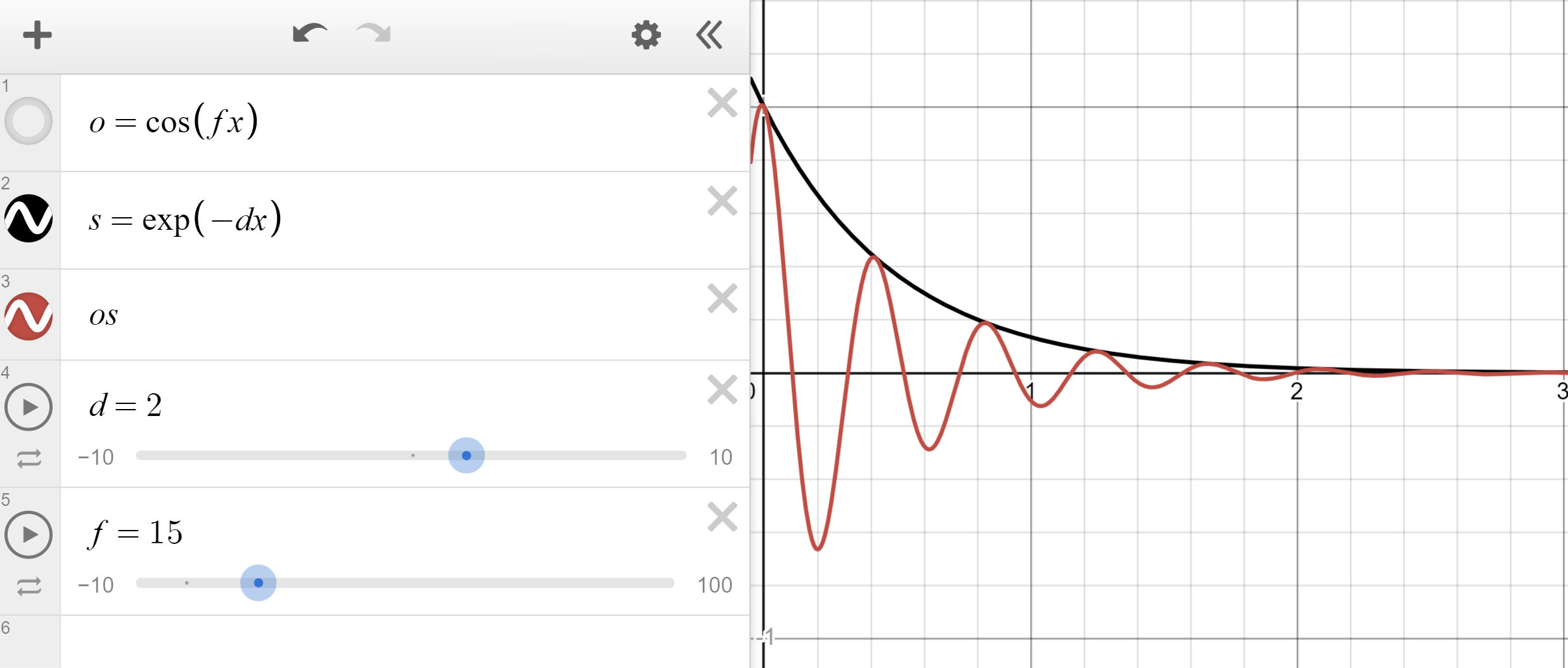
Note how it travels from 1 to 0. This makes it perfect to use as a mix factor, for example with lerp.
float spring(float time; float frequency; float damping) {
    return cos(frequency * time) * exp(-damping * time);
}

// Example usage, spring to targetP
v@P = lerp(v@targetP, v@P, spring(f@Time, 10.0, 5.0));
Overshoot occurs since cos ranges between -1 and 1. To fix this, remap cos between 0 and 1 instead.
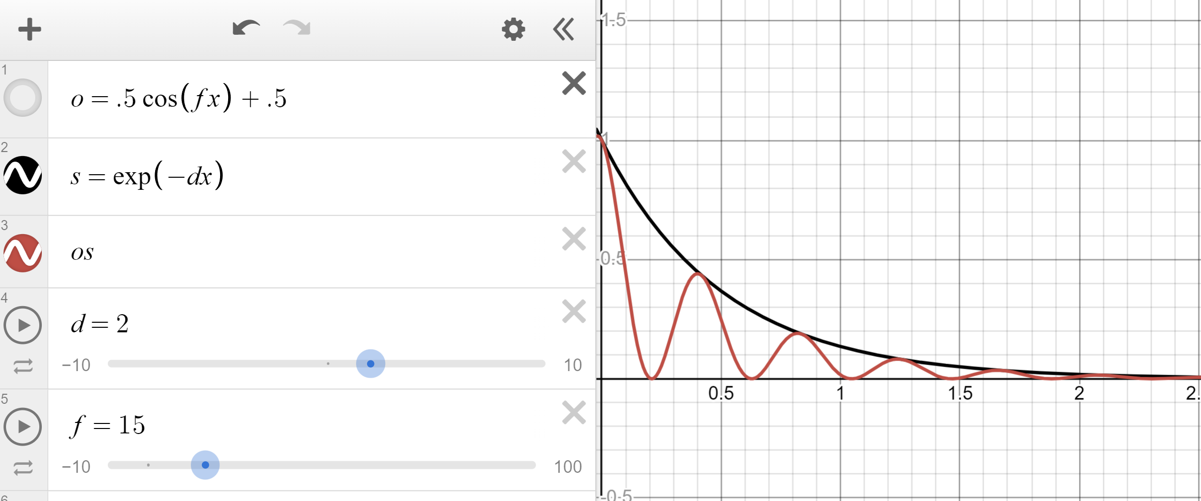
float spring_less(float time; float frequency; float damping) {
    return (cos(frequency * time) * 0.5 + 0.5) * exp(-damping * time); // Or fit11(..., 0, 1)
}

// Example usage, spring to targetP
v@P = lerp(v@targetP, v@P, spring_less(f@Time, 10.0, 5.0));
Make an aimbot (find velocity to hit a target)
Want to prepare for the next war but can’t solve projectile motion? Never fear, the Ballistic Path node is all you need.

| Video Tutorial | | — |
Hit a static target
- Connect your projectile to a Ballistic Path node.
- Set the Launch Method to “Targeted” and disable drag.
- Add a
@targetPattribute to your projectile. Set it to the centroid of the target object.
v@targetP = getbbox_center(1);
- You should see an arc. Transfer the velocity of the first point of the arc to your projectile.
v@v = point(1, "v", 0);
-
Connect everything to a RBD Solver.
-
Use “Life” to set the height of the path, and lower the “FPS” to reduce unneeded points.
Hit a moving target
Use the same method as before, but sample the target’s position forwards in time.
- On the Ballistic Path node, set the Targeting Method to “Life”.
- Copy the “Life” attribute. It’s the number of seconds until we hit the target. We need to find where the target is at that time.
- Add a Time Shift node to the target (before the centroid is calculated). Set it to the current time plus the “Life” attribute.
| Download the HIP file! | | — |
Hit multiple targets
Extract multiple centroids and transfer v from each arc. Enable “Path Point Index” on Ballistic Path, blast non-zero indices, then Attribute Copy v.
If your “Life” changes per target, set a life attribute on each point.
Copernicus: Radial Blur
Simple radial blur shader I made for Balthazar on the CGWiki Discord.

#bind layer src? val=0
#bind layer !&dst

#bind parm quality int val=10
#bind parm center float2 val=0
#bind parm scale float val=0.2
#bind parm rotation float val=0

@KERNEL
{
    float2 offset = @P - @center;
    float4 result = 0.;
    float scale = 1;

    for (int i = 0; i <= @quality; ++i) {
        result += @src.imageSample(offset * scale + @center) / (@quality + 1);
        offset = rotate2D(offset, @rotation / @quality);
        scale -= @scale / @quality;
    }

    @dst.set(result);
}
| Download the HIP file! | | — |
Copernicus to Heightfield
Copernicus stores images in 2D volumes. Guess what else is stored in 2D volumes? Heightfields!

| Video Tutorial | | — |
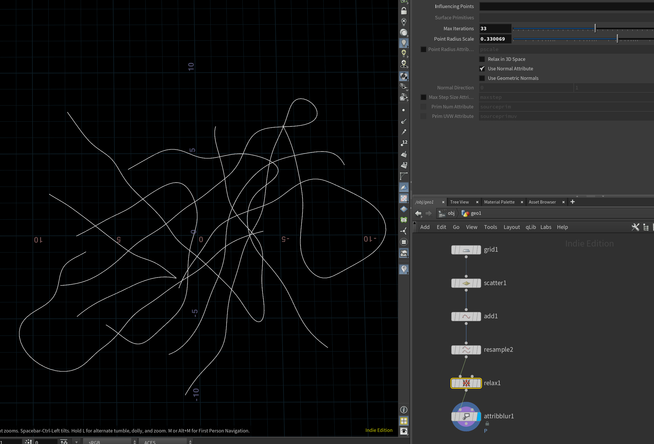
Complex Growth in 2 nodes
You can get cool and organic looking shapes using opposing forces, like Relax and Attribute Blur.

| Download the HIP file! | Video Tutorial | | — | — |
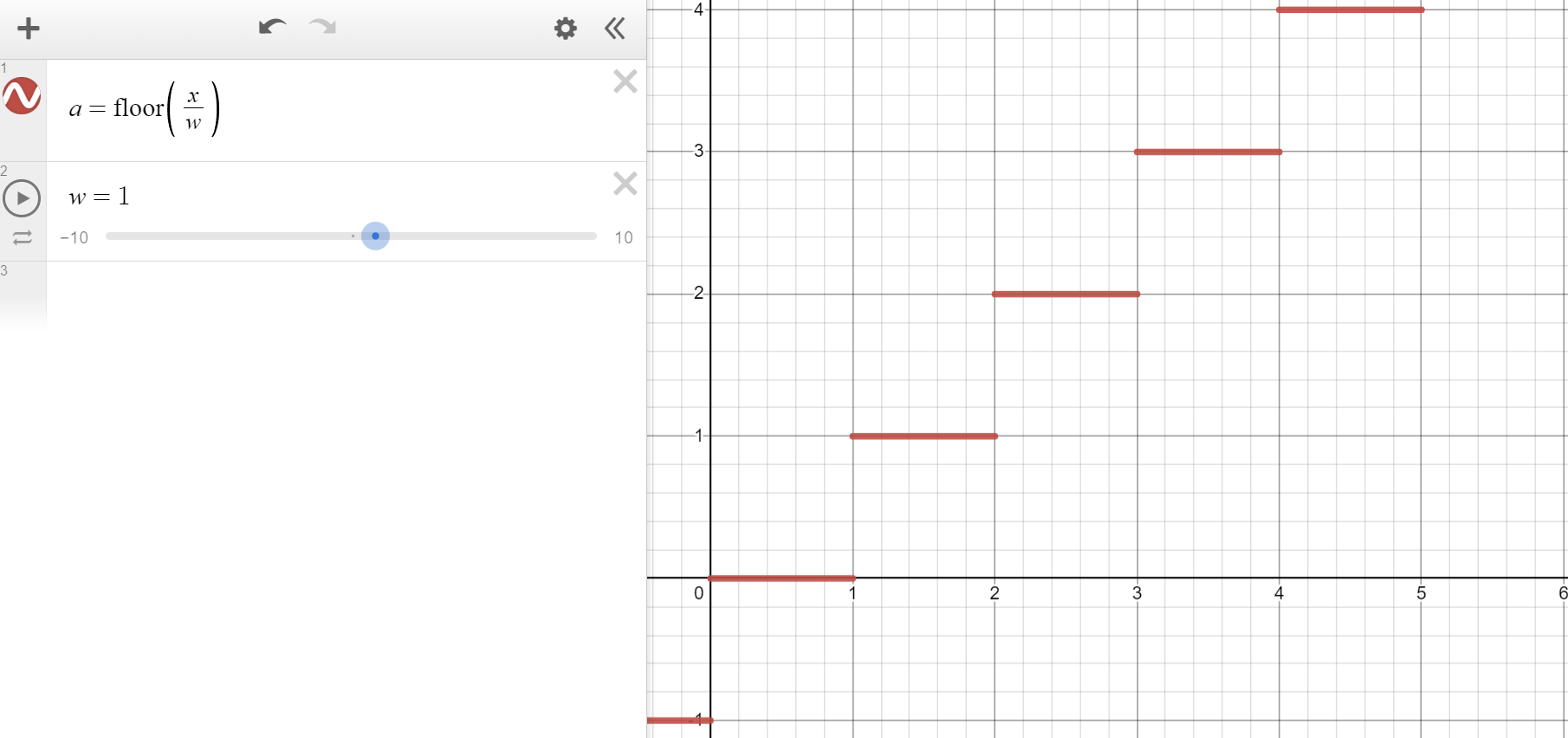
Smooth steps
Smoothstep’s evil uncle, smooth steps. This helps for staggering animations, like points moving along lines.
Start with regular steps. This is the integer component:
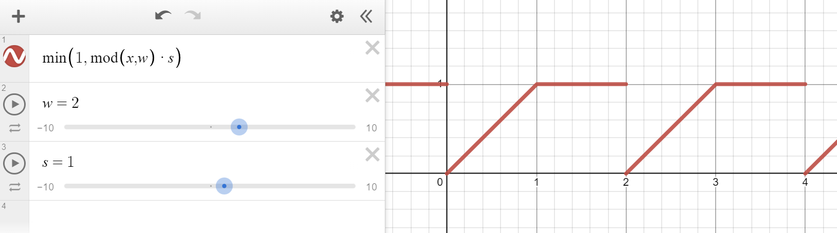
Use modulo to form a line per step, then clamp it below 1. This is the fractional component:
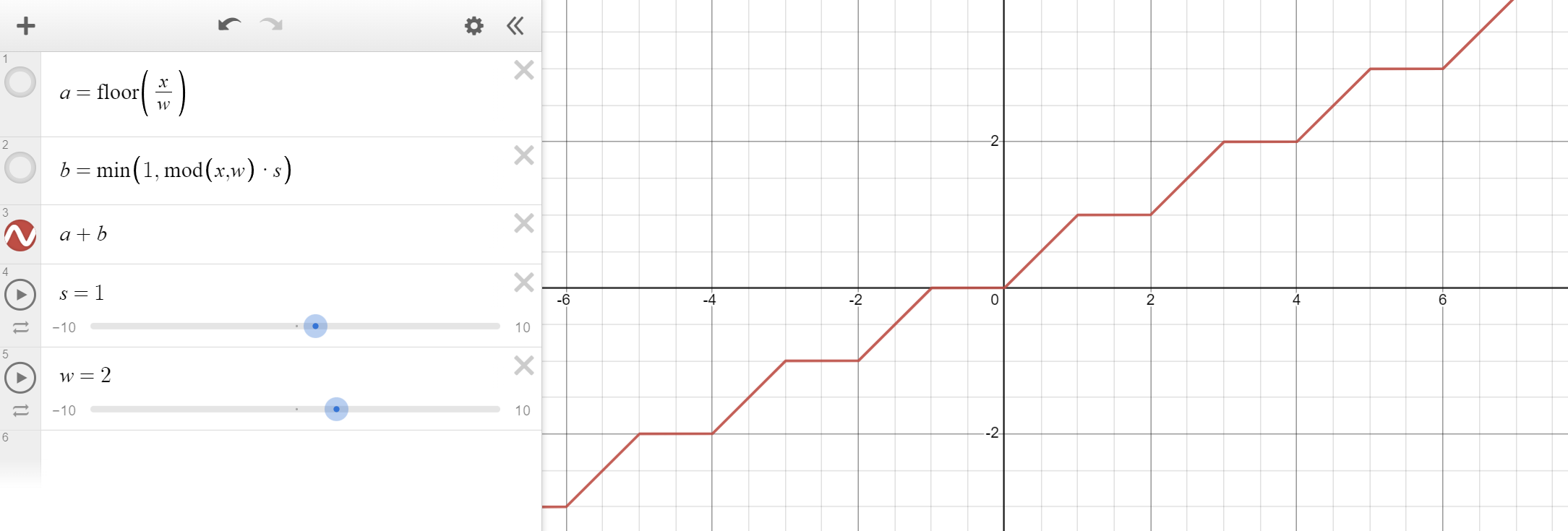
Add them together to achieve smooth steps:
float x = f@Time; // Replace with whatever you want to step
float width = 2; // Size of each step
float steepness = 1; // Gradient of each step

int int_step = floor(x / width); // Integer component, steps
float frac_step = min(1, x % width * steepness); // Fractional component, lines
float smooth_steps = int_step + frac_step; // Both combined, smooth steps
Remove points by time after simulation
Sometimes POP sims take ages to run, especially FLIP sims. This makes it annoying to get notes about timing changes.
I found a decent approach to avoid resimulation:
- Simulate tons of points, way more than you need.
- After simulating, get the birth time of each point using
f@Time - f@age. - Cull points based on the birth time. There’s 2 main ways to do it.
Keyframes over time
chf() lets you fetch values over time using chf("channel", time). Use the birth time and you’re good to go!
float birth_time = f@Time - f@age;
if (chf("keep_percent", birth_time) < rand(i@id)) {
    removepoint(0, i@ptnum, 0);
}
Ramp over time
I used to remap time using a ramp instead. It’s not as controllable as keyframes, but helps in some cases.
float birth_time = f@Time - f@age;
float time_factor = invlerp(birth_time, $TSTART, $TEND);
if (chramp("keep_percent", time_factor) < rand(i@id)) {
    removepoint(0, i@ptnum, 0);
}
| Original Sim | Post-Sim Removal |
|---|---|
 |
 |
I used this ramp for the demo above:
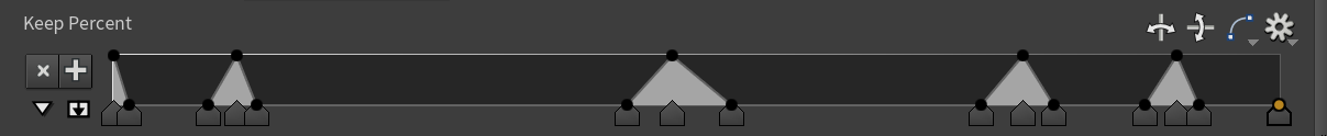
| Download the HIP file! | | — |
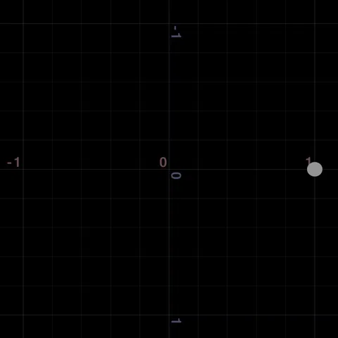
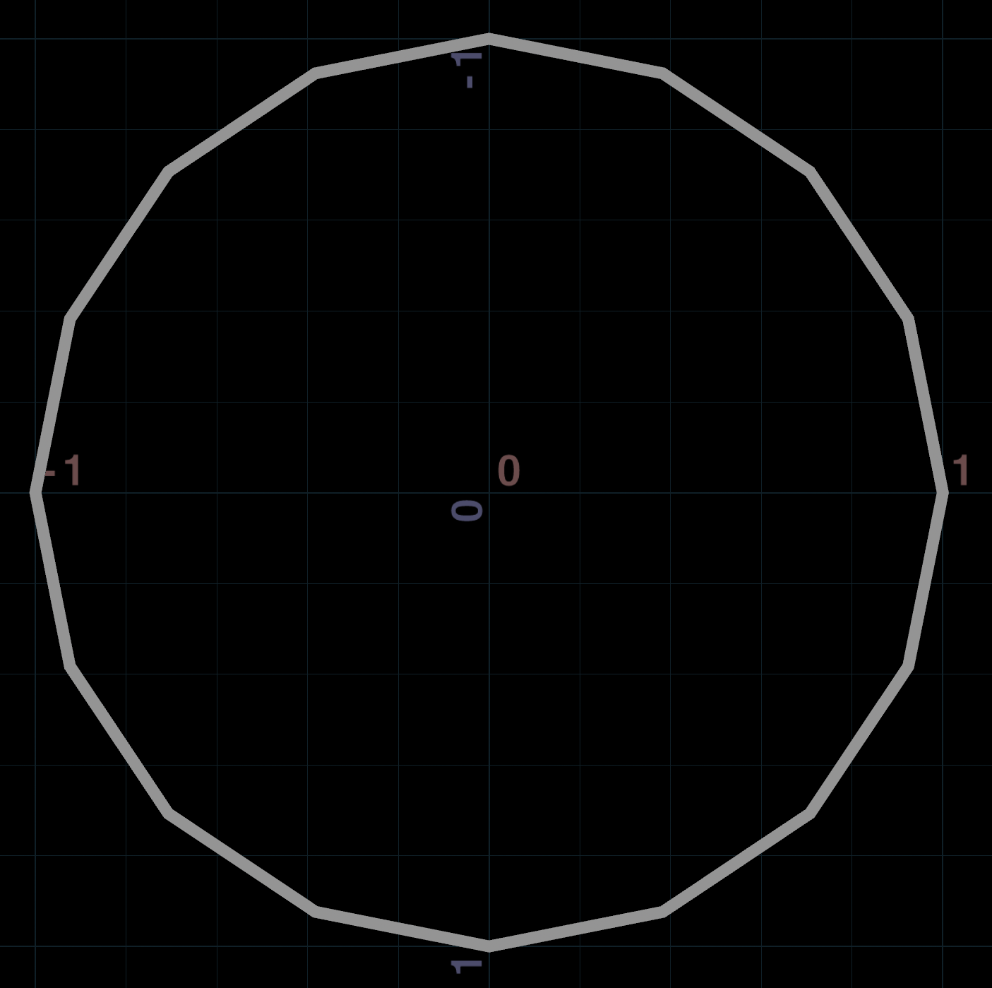
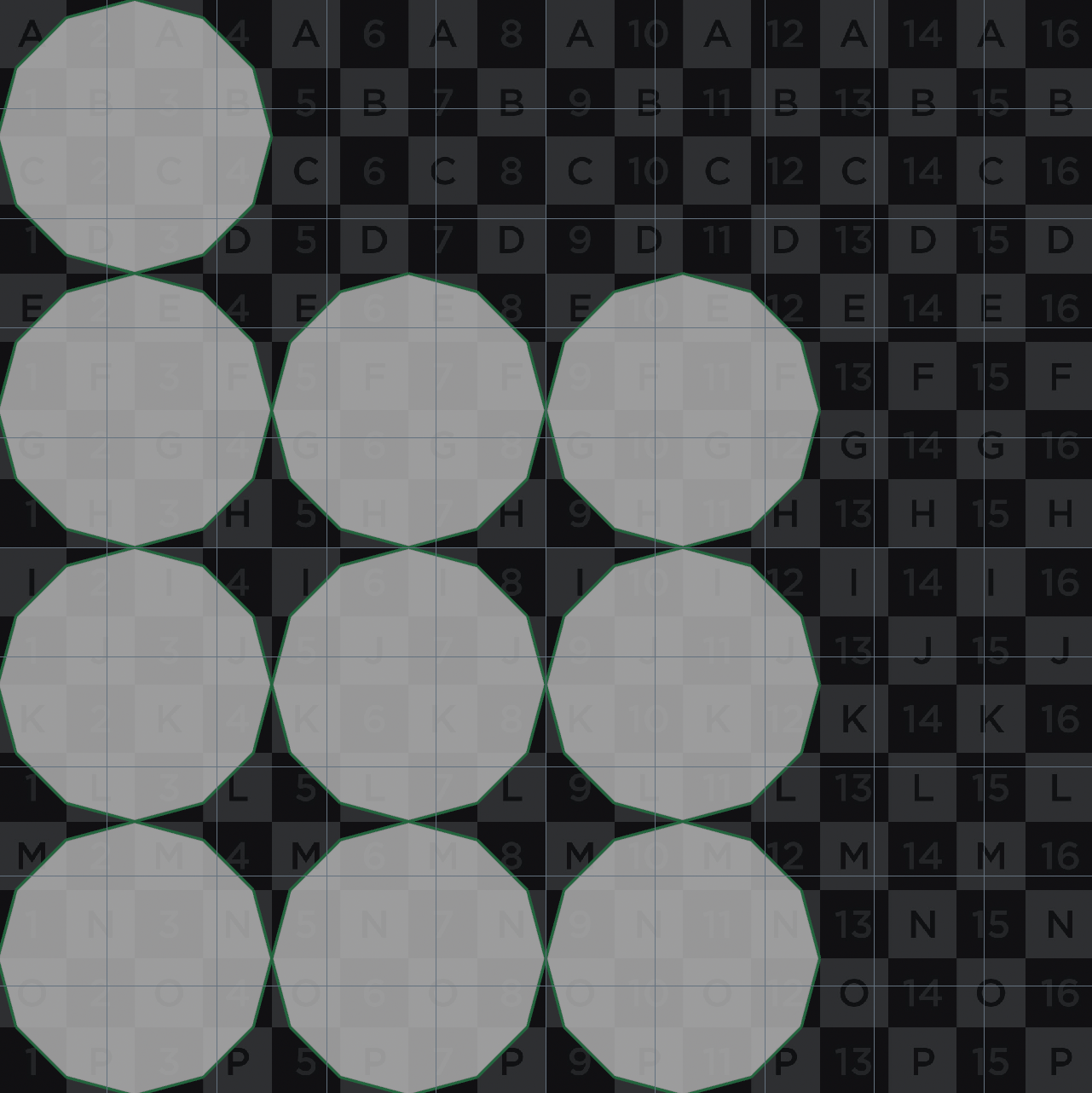
Generating circles
Sometimes you need to generate circles without relying on built-in nodes, like to know the phase.
Luckily it’s easy, just use sin() on one axis and cos() on the other:
float theta = chf("theta");
float radius = chf("radius");
v@P = set(cos(theta), 0, sin(theta)) * radius;
See Waveforms for more about sine and cosine.
To draw a circle, add points while moving between 0 and 2*PI:
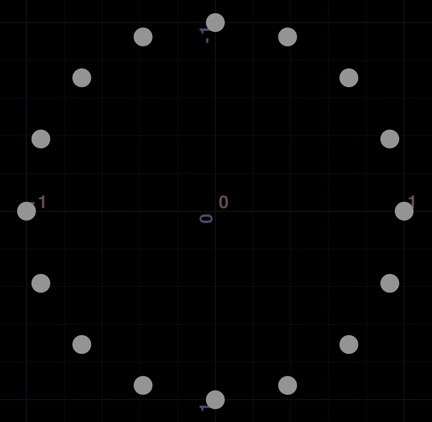
int num_points = chi("point_count");
float radius = chf("radius");

for (int i = 0; i < num_points; ++i) {
    // Sin/cos range from 0 to 2*PI, so remap from 0-1 to 0-2*PI
    float theta = float(i) / num_points * 2 * PI;
    // Use sin and cos on either axis to form a circle
    vector pos = set(cos(theta), 0, sin(theta)) * radius;
    addpoint(0, pos);
}
To connect the points, you can use addprim():
int num_points = chi("point_count");
float radius = chf("radius");
int points[];

for (int i = 0; i < num_points; ++i) {
    // Sin/cos range from 0 to 2*PI, so remap from 0-1 to 0-2*PI
    float theta = float(i) / num_points * 2 * PI;
    // Use sin and cos on either axis to form a circle
    vector pos = set(cos(theta), 0, sin(theta)) * radius;
    // Add the point to the array for polyline
    int id = addpoint(0, pos);
    append(points, id);
}
// Connect all the points with a polygon
addprim(0, "poly", points);
| Download the HIP file! | | — |
Extract Transform in VEX
Ever wondered how Extract Transform works? Turns out it uses a popular matrix solving technique called singular value decomposition.
Align Translation
Aligning the translation is easy. The best translation happens when you align the center of mass (average) of each point cloud.
You don’t even need VEX for this, just use Extract Centroid set to “Center of Mass”, then offset the position by that amount.
// Detail Wrangle: Solves translation only
// Input 1: Source
// Input 2: Target

// 1. Calculate centroids
float n = npoints(1);
vector source_centroid = 0, target_centroid = 0;
for (int i = 0; i < n; ++i) {
    source_centroid += point(1, "P", i);
    target_centroid += point(2, "P", i);
}

// 2. Turn translation into 4x4 matrix
matrix transform = ident();
translate(transform, (target_centroid - source_centroid) / n);

// 3. Add point for Transform Pieces to use
setpointattrib(0, "transform", addpoint(0, {0, 0, 0}), transform);
Align Translation + Rotation
Aligning the rotation is harder. You need to build a covariance matrix, then solve it with SVD.
Luckily we don’t need to leave VEX! Houdini has a SVD solver called svddecomp().
// Detail Wrangle: Solves translation and rotation only
// Input 1: Source
// Input 2: Target

// 1. Calculate centroids
float n = npoints(1);
vector source_centroid = 0, target_centroid = 0;
for (int i = 0; i < n; ++i) {
    source_centroid += point(1, "P", i);
    target_centroid += point(2, "P", i);
}
target_centroid /= n;
source_centroid /= n;

// 2. Build covariance matrix
matrix3 covariance = ident();
for (int i = 0; i < n; ++i) {
    vector source_diff = point(1, "P", i) - source_centroid;
    vector target_diff = point(2, "P", i) - target_centroid;
    covariance += outerproduct(target_diff, source_diff);
}

// 3. Solve rotation with SVD
matrix3 U;
vector S;
matrix3 V;
svddecomp(covariance, U, S, V);
matrix3 R = V * transpose(U);

// 4. Flip if determinant is negative (this causes negative scales to screw up)
if (determinant(R) < 0) {
    R = V * diag({1, 1, -1}) * transpose(U);
}

// 5. Combine translation and rotation into 4x4 matrix
matrix transform = set(R);
translate(transform, target_centroid - source_centroid);

// 6. Add point for Transform Pieces to use
setpointattrib(0, "transform", addpoint(0, {0, 0, 0}), transform);
Align Translation + Rotation + Scale
Aligning the scale is even harder. One popular way is the Umeyama algorithm.
Sadly it only solves uniform scale, and breaks on negative scales. This happens when you flip the sign of the 2nd column of the rotation matrix.
Extract Transform set to “Uniform Scale” also breaks with negative scales, so it probably uses this method!
// Detail Wrangle: Solves translation, rotation, uniform scale (like Eigen::umeyama)
// Input 1: Source
// Input 2: Target

// 1. Calculate centroids
float n = npoints(1);
vector source_centroid = 0, target_centroid = 0;
for (int i = 0; i < n; ++i) {
    source_centroid += point(1, "P", i);
    target_centroid += point(2, "P", i);
}
target_centroid /= n;
source_centroid /= n;

// 2. Build covariance matrix
float deviation = 0;
matrix3 covariance = ident();
for (int i = 0; i < n; ++i) {
    vector source_diff = point(1, "P", i) - source_centroid;
    vector target_diff = point(2, "P", i) - target_centroid;
    deviation += length2(source_diff);
    covariance += outerproduct(target_diff, source_diff);
}

// 3. Solve rotation with SVD
matrix3 U;
vector S;
matrix3 V;
svddecomp(covariance, U, S, V);
matrix3 R = V * transpose(U);

// 4. Flip if determinant is negative (this causes negative scales to screw up)
float det = determinant(R);
vector e = set(1, 1, det < 0 ? -1 : 1);
if (det < 0) {
    R = V * diag(e) * transpose(U);
}

// 5. Solve scale using standard deviation
R *= dot(S, e) / deviation;

// 6. Combine translation rotation and scale into 4x4 matrix
matrix transform = set(R);
translate(transform, target_centroid - (R * source_centroid));

// 7. Add point for Transform Pieces to use
setpointattrib(0, "transform", addpoint(0, {0, 0, 0}), transform);
| Download the HIP file! | | — |
Sweep in VEX
Ever wanted to remake Sweep in VEX? Me neither, but let’s do it anyway!
First we need to know the orientation of each point along the curve.
The easiest way is with the Orientation Along Curve node. Enable the X and Y vectors @out and @up.
The @out and @up vectors define a 3D plane we can slap circles on.
For example, multiply sin() by one vector and cos() by the other, then add them together. This gets a point around a circle flattened to the plane.
v@P += sin(phase) * v@up - sin(phase) * v@out;
Using that in a for loop, we can replace each point with a correctly oriented circle.
int cols = chi("columns");
float radius = chf("radius");
float angle = radians(chf("angle"));

for (int i = 0; i < cols; ++i) {
    // Column factor (0-1 exclusive)
    float col_factor = float(i) / cols;
    // Row factor (0-1 inclusive)
    float row_factor = float(i@ptnum) / (i@numpt - 1);

    // Scale and rotation ramps
    float scale_ramp = chramp("scale_ramp", row_factor);
    float roll_ramp = chramp("roll_ramp", row_factor);

    // Generate circles on the plane defined by v@out and v@up
    float phase = 2 * PI * (col_factor + roll_ramp) + angle;
    vector offset = cos(phase) * v@out - sin(phase) * v@up;

    addpoint(0, v@P + offset * radius * scale_ramp);
}

// Remove original points
removepoint(0, i@ptnum);
Now we just need to connect the circles with quads. To make a quad, we need the index of each corner.
The tricky bit is looping back to the start after we reach the end of each ring, which takes a bit of modulo.
int cols = chi("columns");

// Skip last connections when path is open
int closed = chi("close_path");
if (!closed && i@ptnum >= i@numpt - cols) return;

// Row and column indexes per point
i@ptrow = i@ptnum / cols;
i@ptcol = i@ptnum % cols;

// Point indexes of the 4 corners of each quad
int corner1 = i@ptnum;
int corner2 = i@ptrow * cols + (i@ptnum + 1) % cols;
int corner3 = (corner2 + cols) % i@numpt;
int corner4 = (corner1 + cols) % i@numpt;

// Add quads
int prim_id = addprim(0, "poly", corner1, corner2, corner3, corner4);

// Row and column indexes per prim
setprimattrib(0, "primrow", prim_id, i@ptrow);
setprimattrib(0, "primcol", prim_id, i@ptcol);
The same code works for custom cross sections, though it’s easier to use Copy to Points to orient each cross section.
Just make sure the points are sorted and cols matches the point count of the cross section!
If cols doesn’t match the point count, never fear. You’ll get cool trippy looking shapes!
| Download the HIP file! | | — |
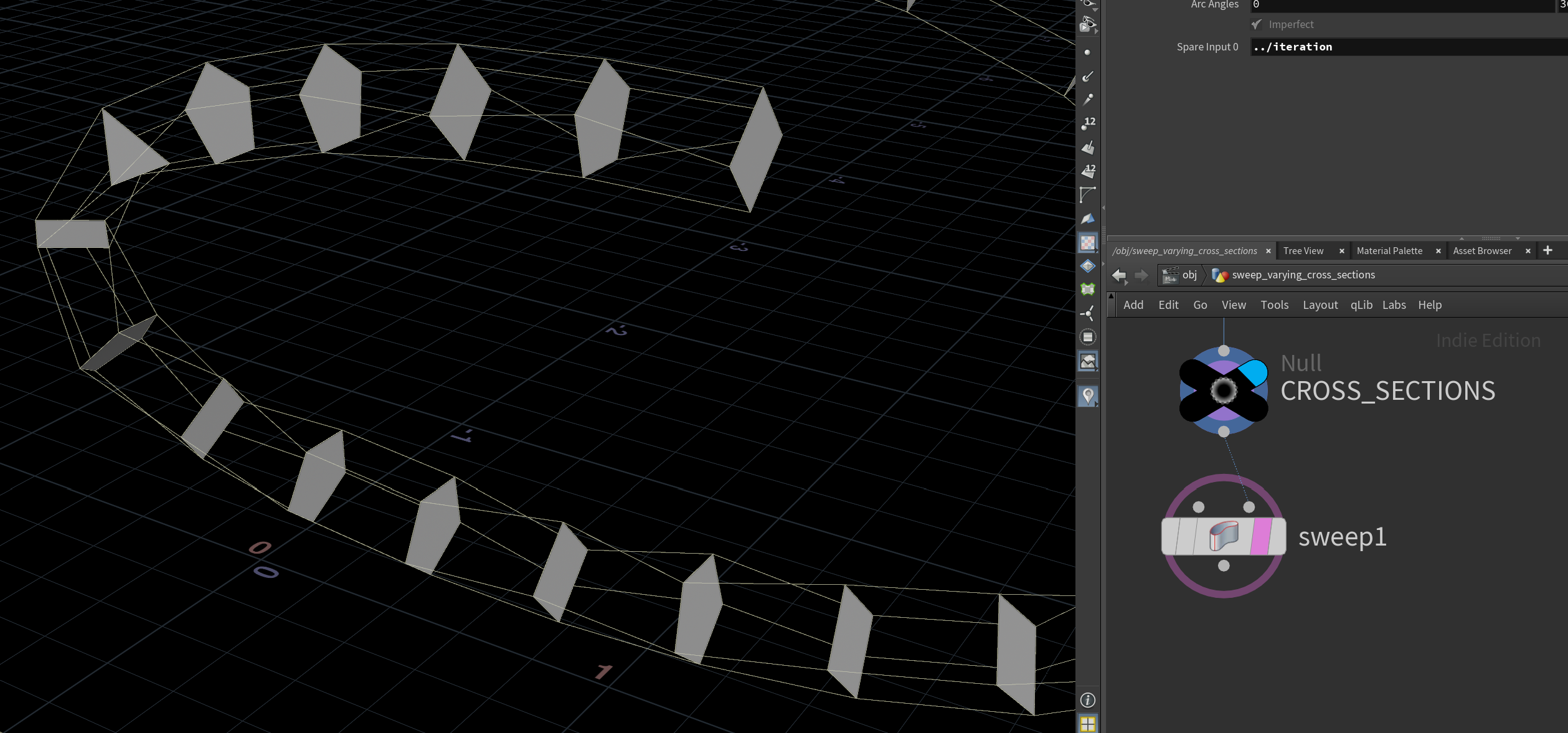
Sweep varying cross sections
I showed this to Lara Belaeva, who pushes Sweep to its limits on LinkedIn. She tried it already, but had an interesting point:
If I decided to build my own Sweep I would try to do it similar to what we have in Plasticity. In Plasticity you can take several different cross-sections, put them in different regions of the curve, and the Sweep creates the blends between them across the curve. I tried to make such a tool but it’s still so-so. Houdini’s Sweep also can use different cross sections, but doesn’t create blends between them
It would be cool if Sweep supported different cross sections. But what if it does already?
Try using normals from Orientation Along Curve, then copy different cross sections onto each point with Copy to Points.
Plug that into Sweep’s second input and you’ll see we can use different cross sections after all!
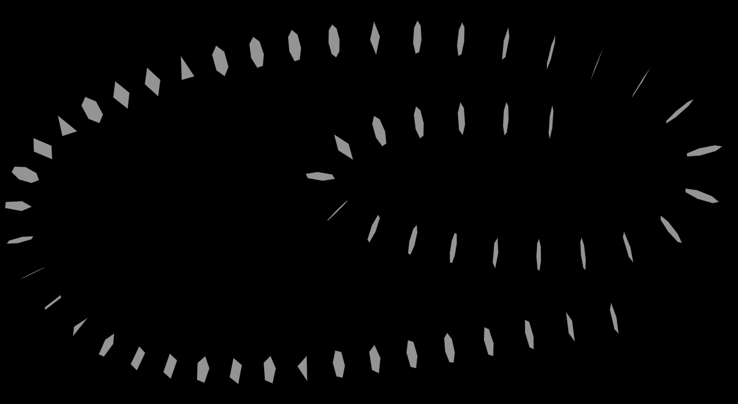
Although it works, if you look closely it resampled each cross section to the same number of points. Lara tried this too:
I just resampled these cross-sections with a constant number of points and then they were sort of placed along the curve based on curveu attribute, and then the algorithm connected 1-1-1, 2-2-2, 3-3-3 points of these cross-sections with polylines. And then these polylines were turned into a mesh with Loft.
So what if we want the exact same cross sections? PolyBridge comes to our rescue!
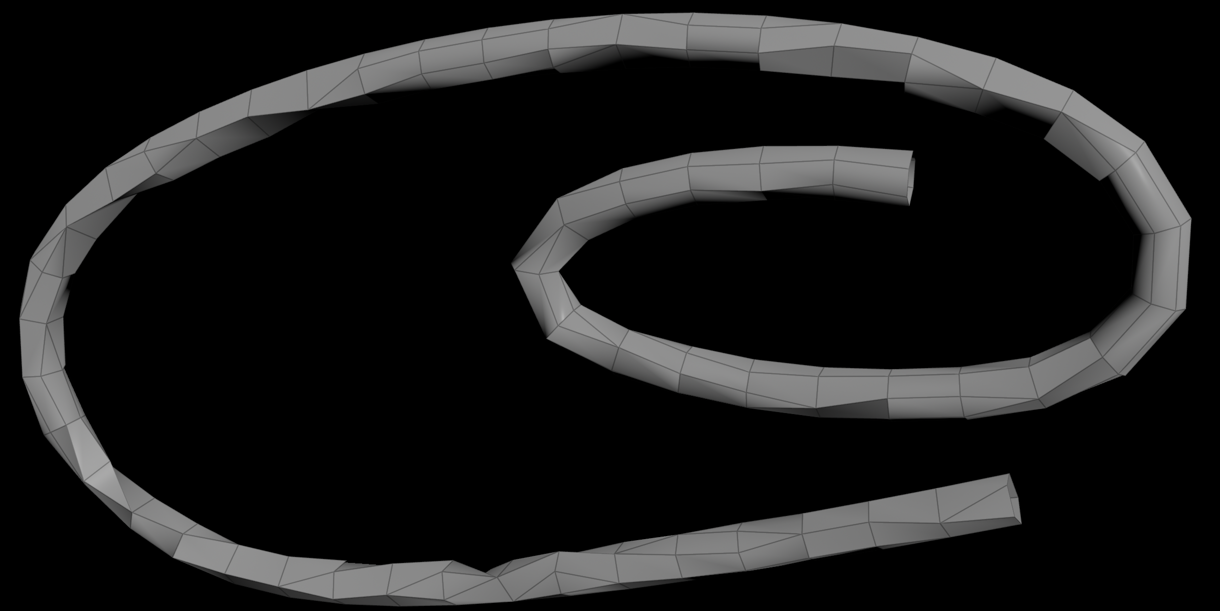
Plug the cross sections into a PolyBridge node instead. Set the source group to all prims from 0 to the second last:
0-`nprims(0)-2`
Set the destination group to all prims from 1 to the last:
1-`nprims(0)-1`
Now the cross sections connect perfectly without any resampling!
| Download the HIP file! | | — |
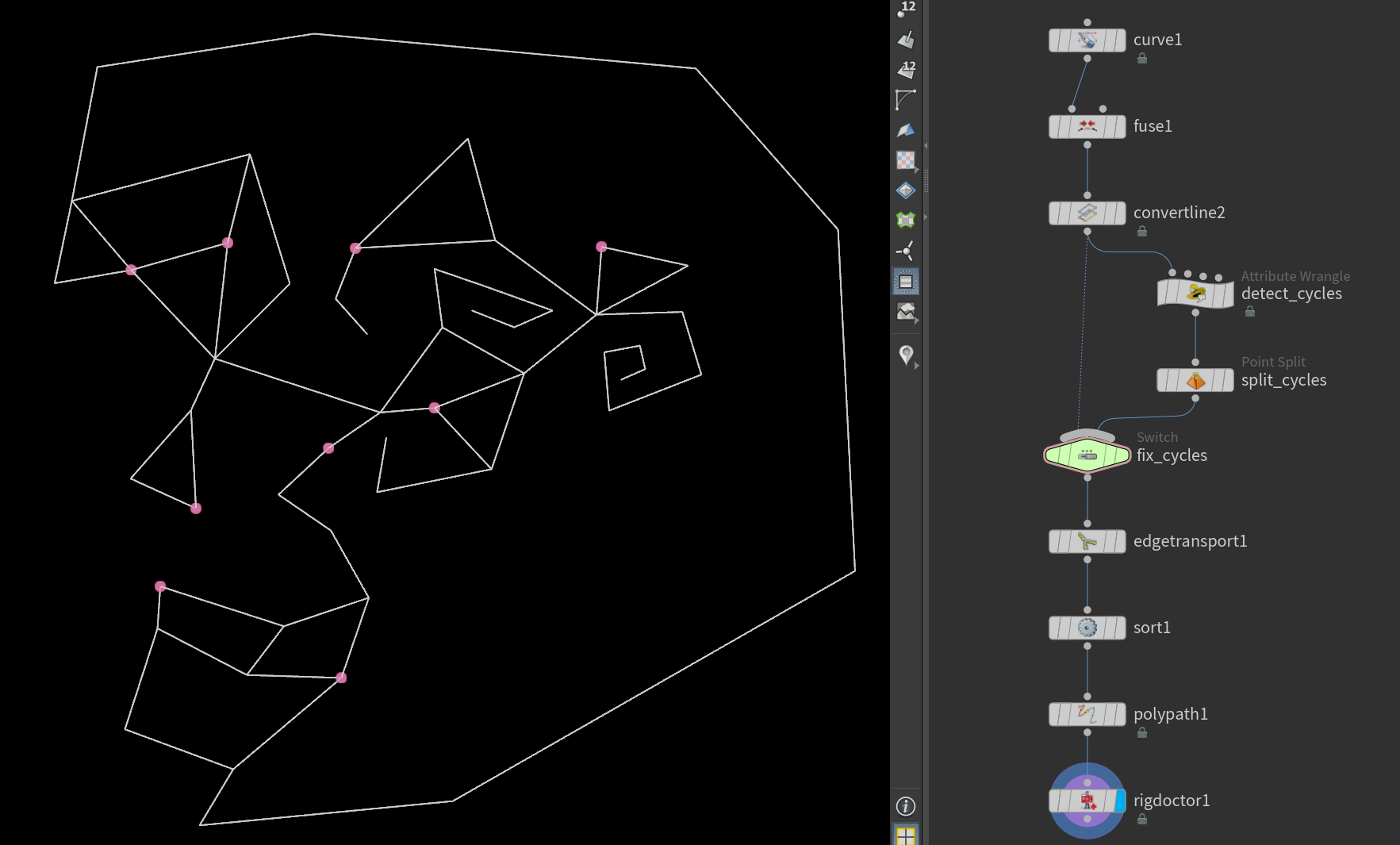
KineFX: Detect and Fix Cyclic Skeletons
KineFX often whinges when skeletons are cyclic. There’s a good section on CGWiki to fix this, but it only works if there truly aren’t cycles.
If the skeleton actually has cycles, you’ll need to detect cycles and cut them. I couldn’t find a node for this, so I used VEX.
// Depth first search to detect graph cycles for cutting
int n = i@numpt;
int sums[];
resize(sums, n);
int stack[] = {0};

// Also check if the stack is empty in case the final point has a cycle
for (int i = 0; i < n || len(stack) > 0; ++i) {

  // Get the next point in the stack, or whatever point hasn't been visited yet
  int current = len(stack) > 0 ? pop(stack, 0) : find(sums, 0);

  // If we've seen this point already, we found a cycle
  if (++sums[current] > 1) {
    // Group it to be split
    setpointgroup(0, "cyclic", current, 1);
    // Add an iteration since we skipped this one
    ++n;
    continue;
  }

  // Add all the neighbours we haven't explored to the stack
  foreach (int next; neighbours(0, current)) {
    if (sums[next] == 0) insert(stack, 0, next);
  }
}
I tried using PolyCut, but it doesn’t cut all connections. Convert Line and Point Split seems to work though.
| Download the HIP file! | | — |
Fitting UV islands
Sometimes you need to overlap UV islands and fit them to a full tile, like when slicing a sphere.
This is hard to do with Houdini’s built-in nodes, so here’s a manual approach.
- Use Attribute Promote to get the min and max of the UV attribute. If there’s multiple islands, go per piece by connectivity.
- Use a Vertex Wrangle to manually fit the UVs based on the min and max.
v@uv = invlerp(v@uv, v@uvmin, v@uvmax); // Or v@uv = fit(v@uv, v@uvmin, v@uvmax, 0, 1);
| Before | After |
|---|---|
 |
 |
| Download the HIP file! | | — |
Reusing code in multiple wrangles
Most programming languages have ways to share and reuse code. C has #include, JavaScript has import, but what about VEX?
VEX has #include as well, but sadly it only works if you put the file in a specific Houdini directory.
Luckily there’s a secret way to reuse code without #include! I found it in a couple of LABS nodes.
First add any node with a string property. It can be a wrangle, a null or anything else. In the string property, type the functions you want to share.
vector addToPos(vector p) {
    return p + {1, 2, 3};
}
Now you can import and run those functions in any other wrangle with chs("../path/to/string_property") enclosed in backticks!
// Append the code string and run it (like #include)
`chs("../path/to/string_property")`

v@P = addToPos(v@P);
UPDATE: Van and WaffleboyTom said this is evil since it causes the code to recompile. Use if you dare!
| Download the HIP file! | | — |
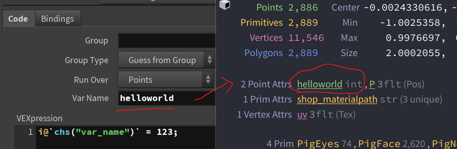
Dynamic attribute names
A similar hack is using chs("var_name") to set an attribute name at compile time.
For example, making a dynamically named integer attribute set to 123:
i@`chs("var_name")` = 123;
Certain characters like spaces aren’t allowed in variable names, so try not to include them!
| Download the HIP file! | | — |
Procedural text in the Font node
Surprisingly it’s tricky to display text based on an attribute or VEX snippet. Here’s a few ways to do it!
| Download the HIP file! | | — |
Expressions
Igor Elovikov told us about a top secret Houdini feature, multiline expressions!
You can do it in expression but it’s a rather an esoteric part of Houdini parameters.
Multiline expressions must be enclosed in {} and have a return statement, otherwise they evaluate to zero.
`{
string result = '';
for (i = 0; i < 10; i++) {
    result = strcat(result, 'any');
}
return result;
}`
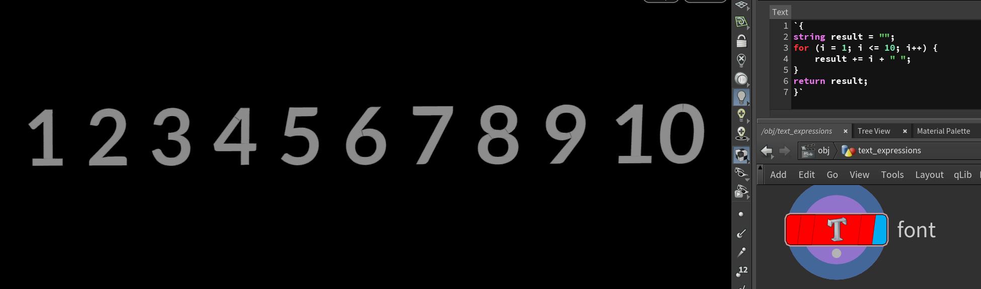
Igor used strcat() to join the strings. I found adding works too, it doesn’t need typecasting unlike VEX!
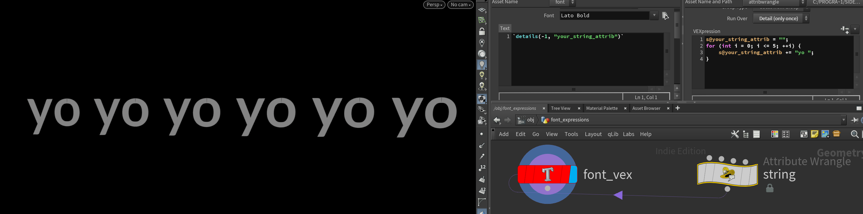
Detail attribute
If you want to use VEX, never fear! Make a detail attribute, add it as a spare input, then use details() to display it as text.
`details(-1, "your_string_attrib")`
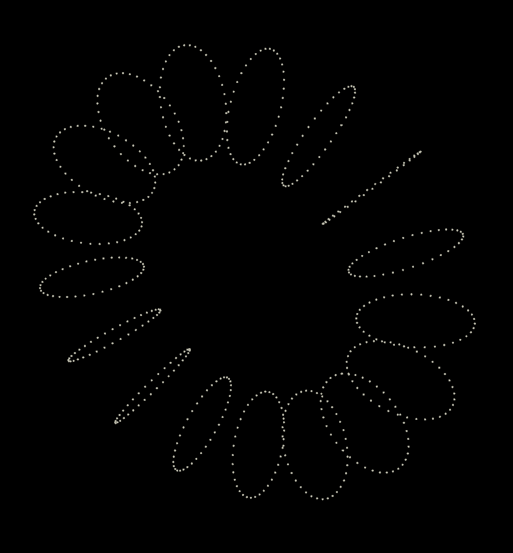
Overlapping cables without intersection
Vladimir on the CGWiki Discord wanted to generate random curves and stop them from intersecting.
Start by scattering a bunch of points and connecting every few using an Add node. This makes a bunch of random lines.
Now let’s smooth them out. You can Resample, Blur, or Convert them to NURBS or Bezier paths. Use Relax to spread them out too.
To stop intersection a Vellum sim is likely the best, though I found Vellum Post Process and Relax work well too.
The key is making sure the points aren’t coplanar, otherwise they spread in 2D only. Randomize the position a little first, then use Vellum Post Process or Relax.
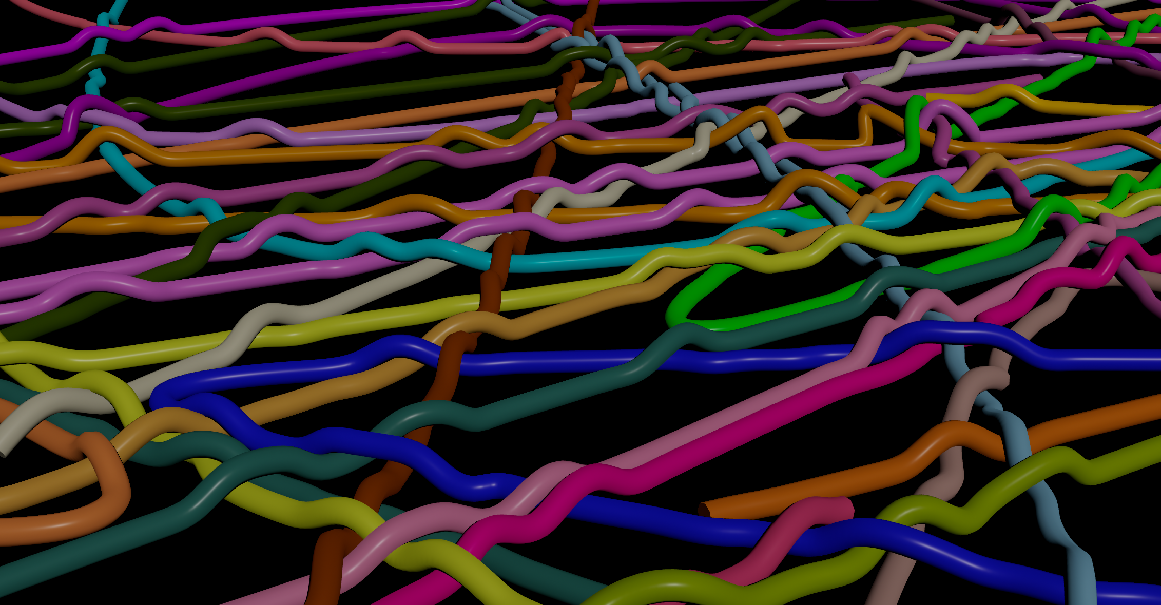
| Download the HIP file! | | — |
Nearest point to any attribute
nearpoint() finds the closest point to @P, but what if you need the closest point to something else?
The shortest way is abusing pcfind(), which takes any input as the position channel:
string attrib = "density";
float target = 16.0;
int nearest_id = pcfind(0, attrib, target, 99999.9, 1)[0];
Another option is using Attribute Swap to move the attribute to @P. Keep in mind this only works for certain types of attributes.
To find an exact match, use findattribval() instead.
Unwrap
Swalsch told us about a top secret alternative to the above, known as unwrap.
It changes the context of any VEX function, allowing you to override functions to work with any attribute.
For example, nearpoint() uses @P. Normally you have to round trip to use another attribute like @uv:
// Get the geometry position closest to a UV coordinate
vector world_pos = uvsample(0, "P", "uv", chv("uv_coordinate"));

// Find the nearest point to that position
i@near_id = nearpoint(0, world_pos);
The direct way is using unwrap to replace the context:
// All in one, thanks @swalsch!
i@near_id = nearpoint("unwrap:uv opinput:0", chv("uv_coordinate"));
| Download the HIP file! | | — |
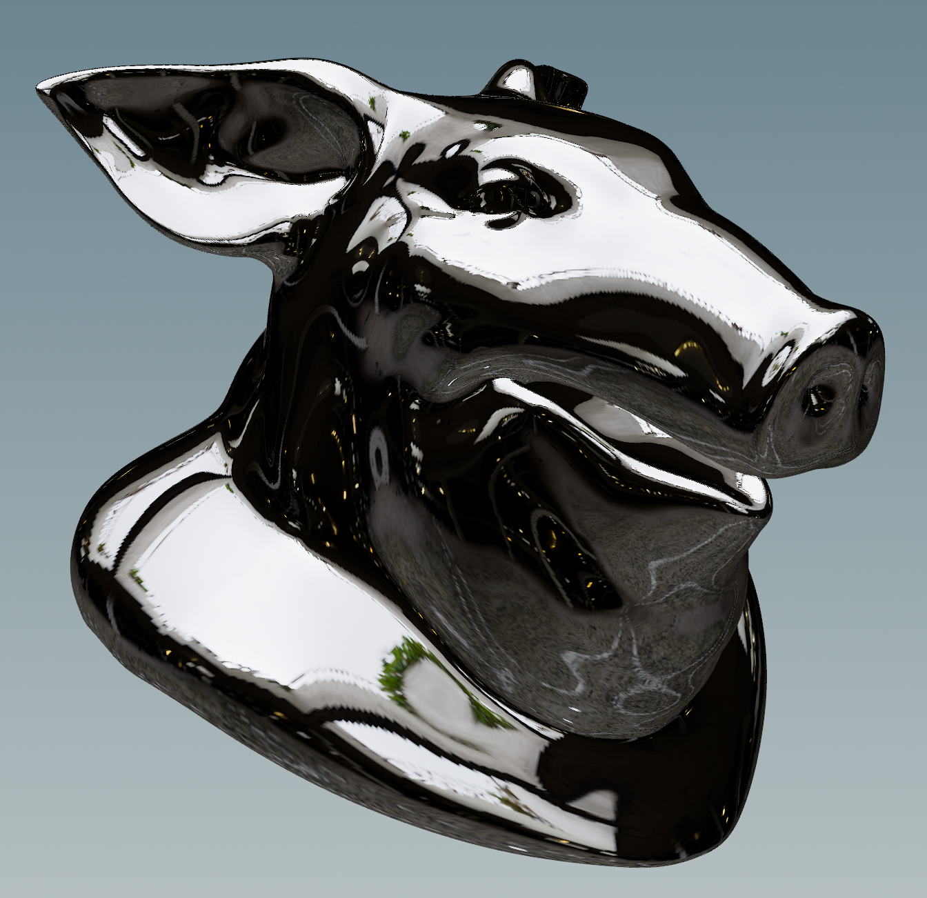
Sampling environment maps
A cool trick from John Kunz is sampling a HDRI using VEX. It’s a cheap way to get environment mapping without leaving the viewport.
// Insert your camera position here
vector cam_pos = fromNDC("/obj/cam1", {0, 0, 0});

// John Kunz magic
vector r = normalize(reflect(normalize(v@P - cam_pos), v@N));
vector uv = set(atan2(-r.z, -r.x) / PI + 0.5, r.y * 0.5 + 0.5, 0);
v@Cd = texture("$HFS/houdini/pic/hdri/HDRIHaven_skylit_garage_2k.rat", uv.x, uv.y);
| Download the HIP file! | | — |
Smoothing volumes with VEX
Levin on the CGWiki Discord wanted to blur volumes in VEX. You can do it by sample neighbors in a box and averaging them together. This is slower than the built-in volume nodes, but might be useful one day:
float density_sum = 0;
int num_samples = 0;

int voxel_radius = chi("voxel_radius");
for (int x = -voxel_radius; x <= voxel_radius; ++x) {
    for (int y = -voxel_radius; y <= voxel_radius; ++y) {
        for (int z = -voxel_radius; z <= voxel_radius; ++z) {
            // Sample voxel at offset index
            vector voxel = set(i@ix + x, i@iy + y, i@iz + z);
            float density = volumeindex(0, 0, voxel);

            // Add to sum and sample count
            density_sum += density;
            ++num_samples;
        }
    }
}

f@density = density_sum / num_samples;
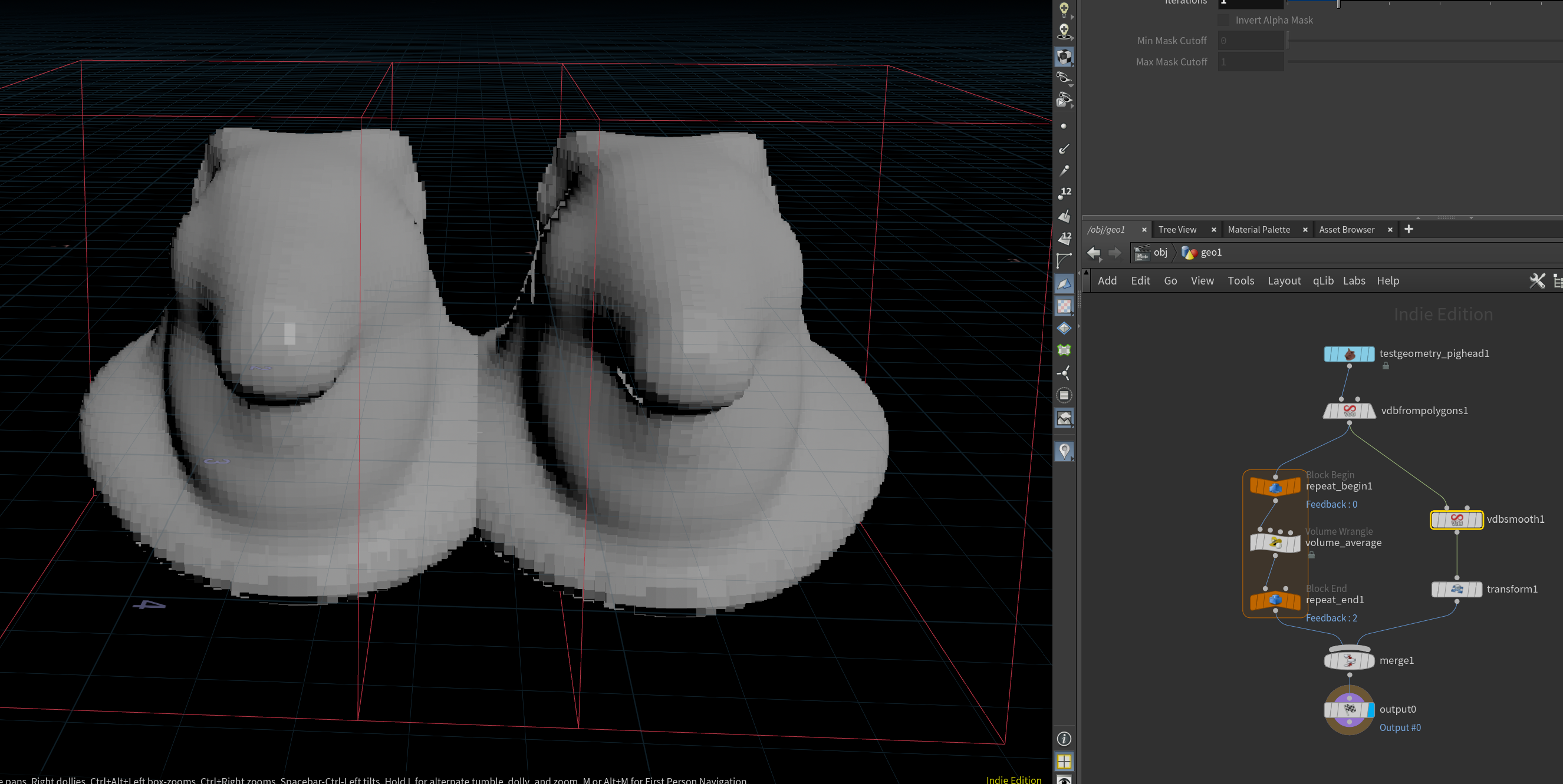
| Download the HIP file! | | — |
Split curve to individual lines and back again
Putting this here since I always forget the nodes.
- “Convert Line” splits a single prim curve into multiple line prims.
- “PolyPath” combines multiple line prims into a single curve prim.
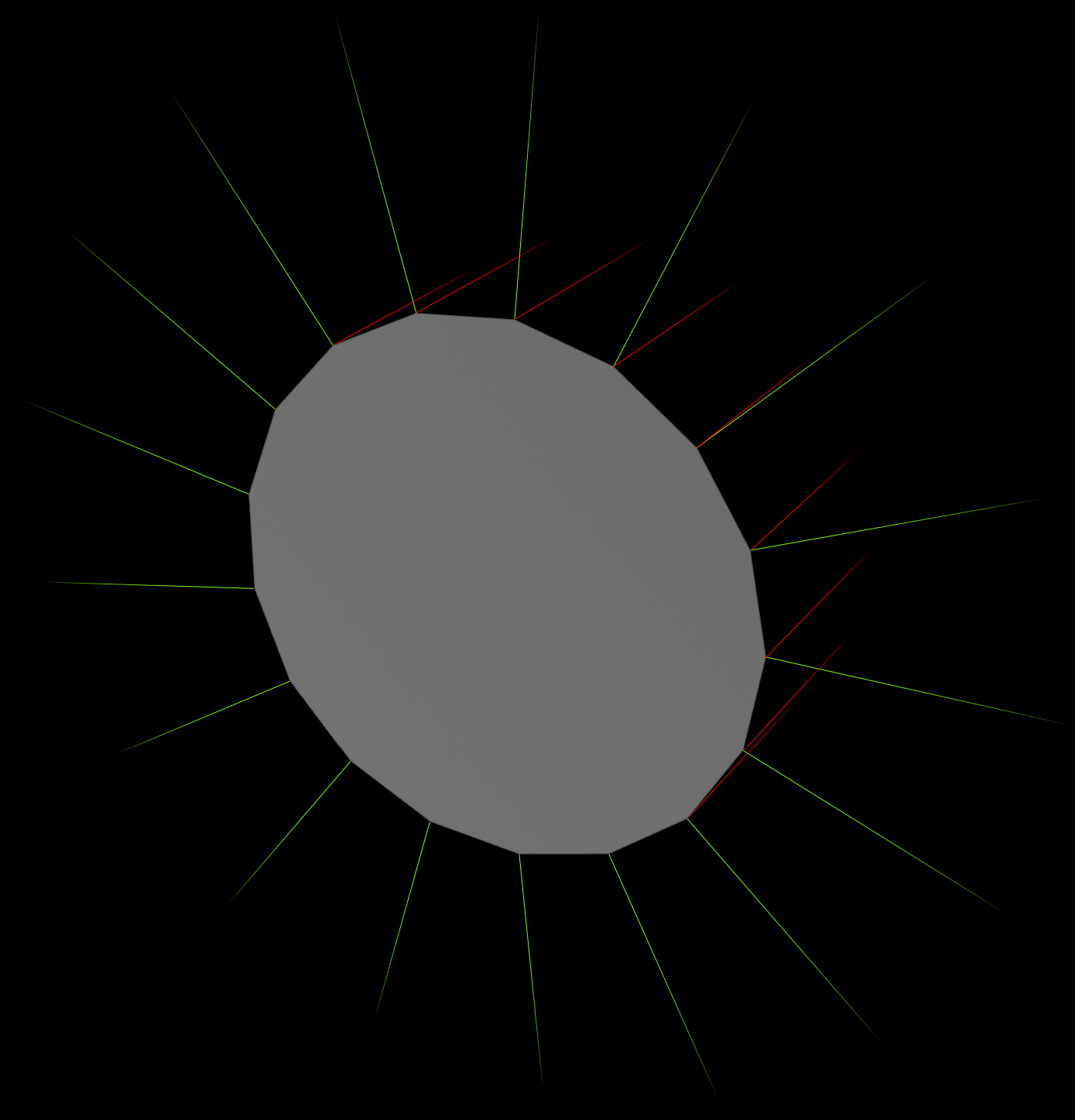
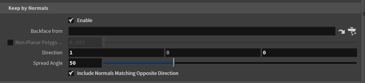
Keep by normals in VEX
The Group node has a useful option to select by normals. Carlll on the CGWiki Discord was looking for a VEX equivalent.
A dot product tells how similar two vectors are, negative when opposite, positive when similar.
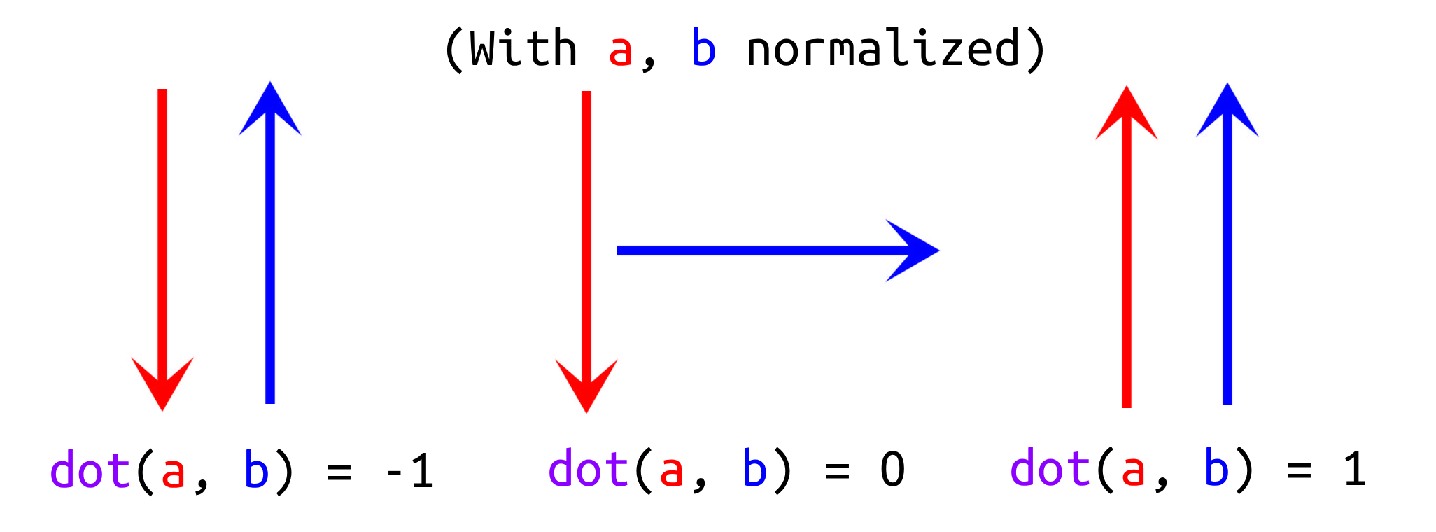
To know if a vector points in a direction, you’d check if the dot product passes a threshold.
@group_upward = dot(v@N, {0, 1, 0}) > chf("threshold");
Here’s a more complete version:
float similarity = dot(v@N, normalize(chv("direction")));
if (chi("include_opposite_direction")) {
    similarity = abs(similarity);
}
i@group_`chs("group_name")` = similarity >= cos(radians(chf("spread_angle")));
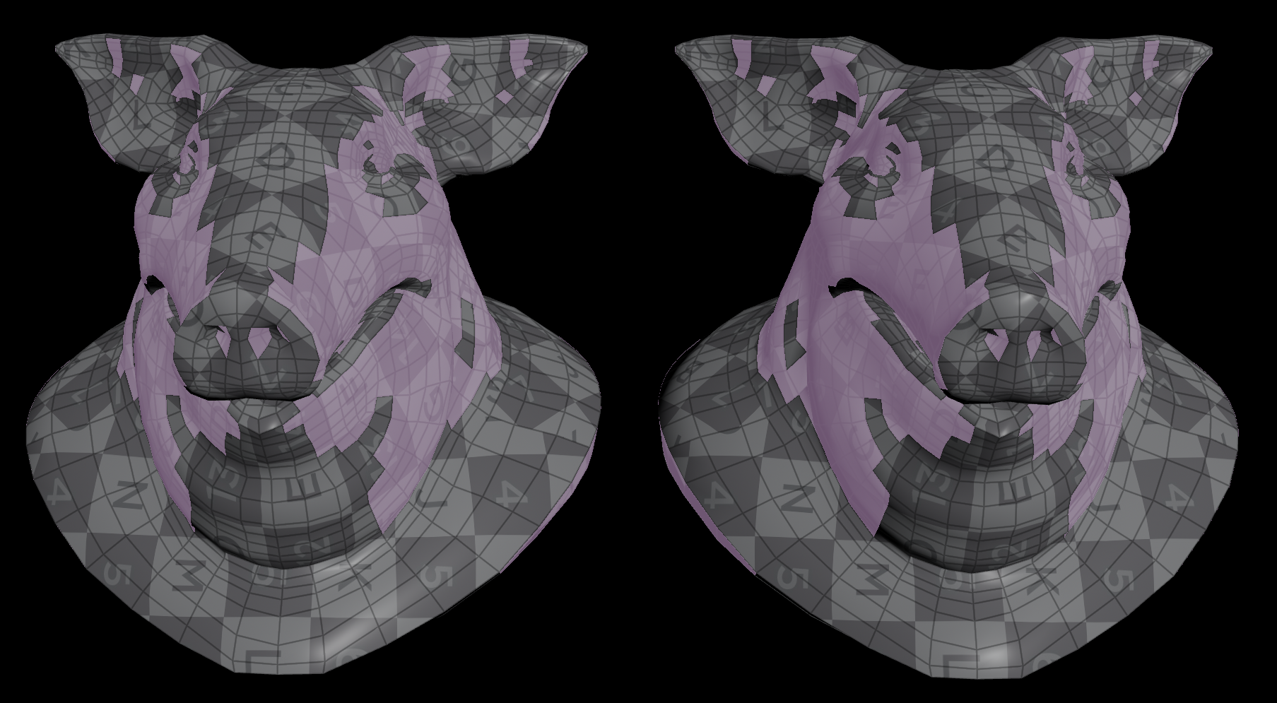
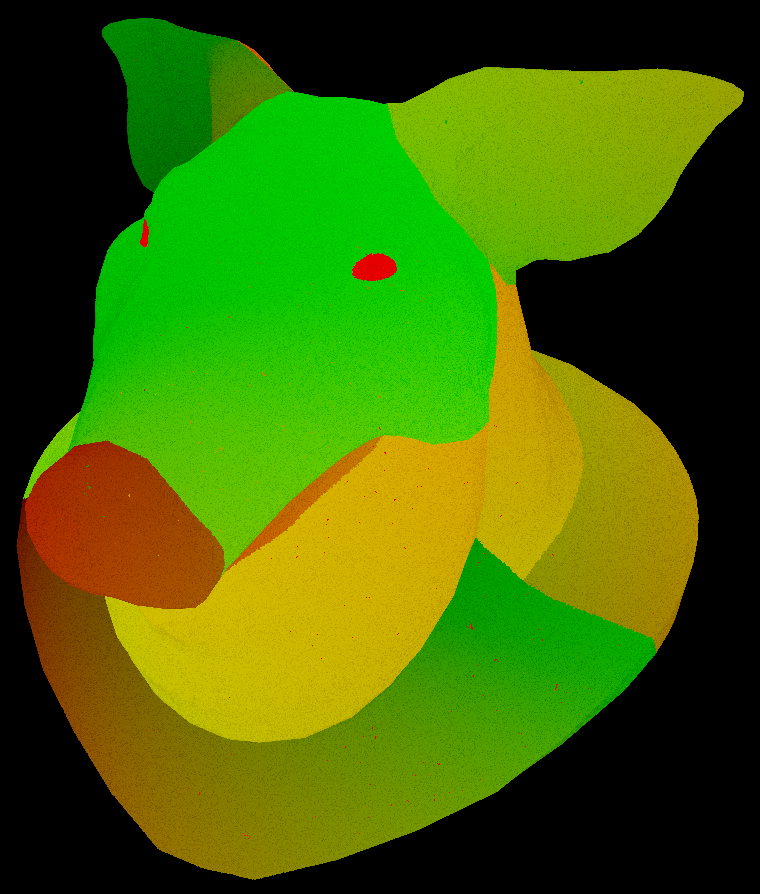
Spot the difference. On the left is the Group node, on the right is VEX.
| Download the HIP file! | | — |
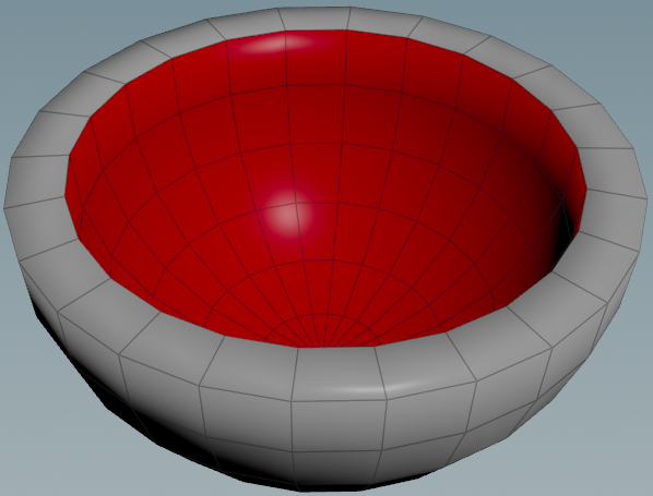
Select inside or outside
Sometimes you need to select the inside or outside of double-sided geometry, for example to make single-sided geometry if Fuse doesn’t work.
The normals are great whenever you need to select anything by direction. Usually you can use a Group node set to “Keep By Normals”, then use “Backface from” to pick the interior.
If it screws up, here’s another approach. Assuming the interior points inwards and the exterior points outwards, the normals of the interior should point roughly towards the center. That means to detect the interior, you can compare the direction of the normal with the direction towards the center.
- Pick a center point. Extract Centroid is good for this.
vector center = point(1, "P", 0);
- Find the direction towards the center.
vector dir = normalize(center - v@P);
- Compare it to the normal using a dot product. This tells you how much the normal faces the center (-1 to 1).
float correlation = dot(dir, v@N);
@group_inside = correlation > ch("threshold");
| Download the HIP file! | | — |
Collision geometry from nasty meshes
It’s always hard to get a decent sim when your collision geometry is on life support. Here’s a few ways to clean it up!
Particle Fluid Surface
Good for point clouds! VDB from Particles works too, but not as smoothly.
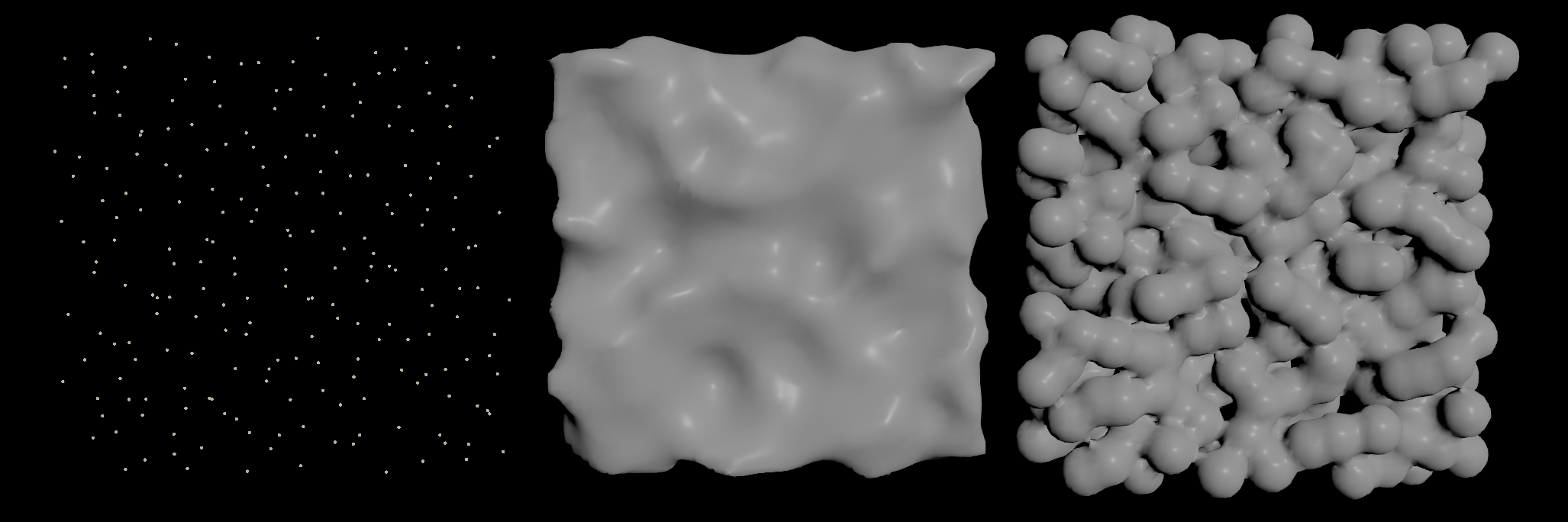
| Download the HIP file! | | — |
Extrude
Good for flat surfaces! For more control, use point normals to set the extrusion direction.
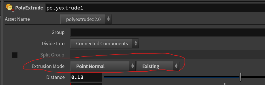
| Download the HIP file! | | — |
Applying orient to packed prims
Copy to Points automatically applies quaternions like @orient, but what if you need the same effect without Copy to Points?
Normally you’d set the transform intrinsic, but this replaces everything. To just replace the @orient, set pointinstancetransform to 1.
setprimintrinsic(0, "pointinstancetransform", i@elemnum, 1);
Thanks to WaffleboyTom for this tip!
Snapping to the floor
Often it’s nice to organise geometry by snapping it to the floor. Here’s a few ways to do it!
| Download the HIP file! | | — |
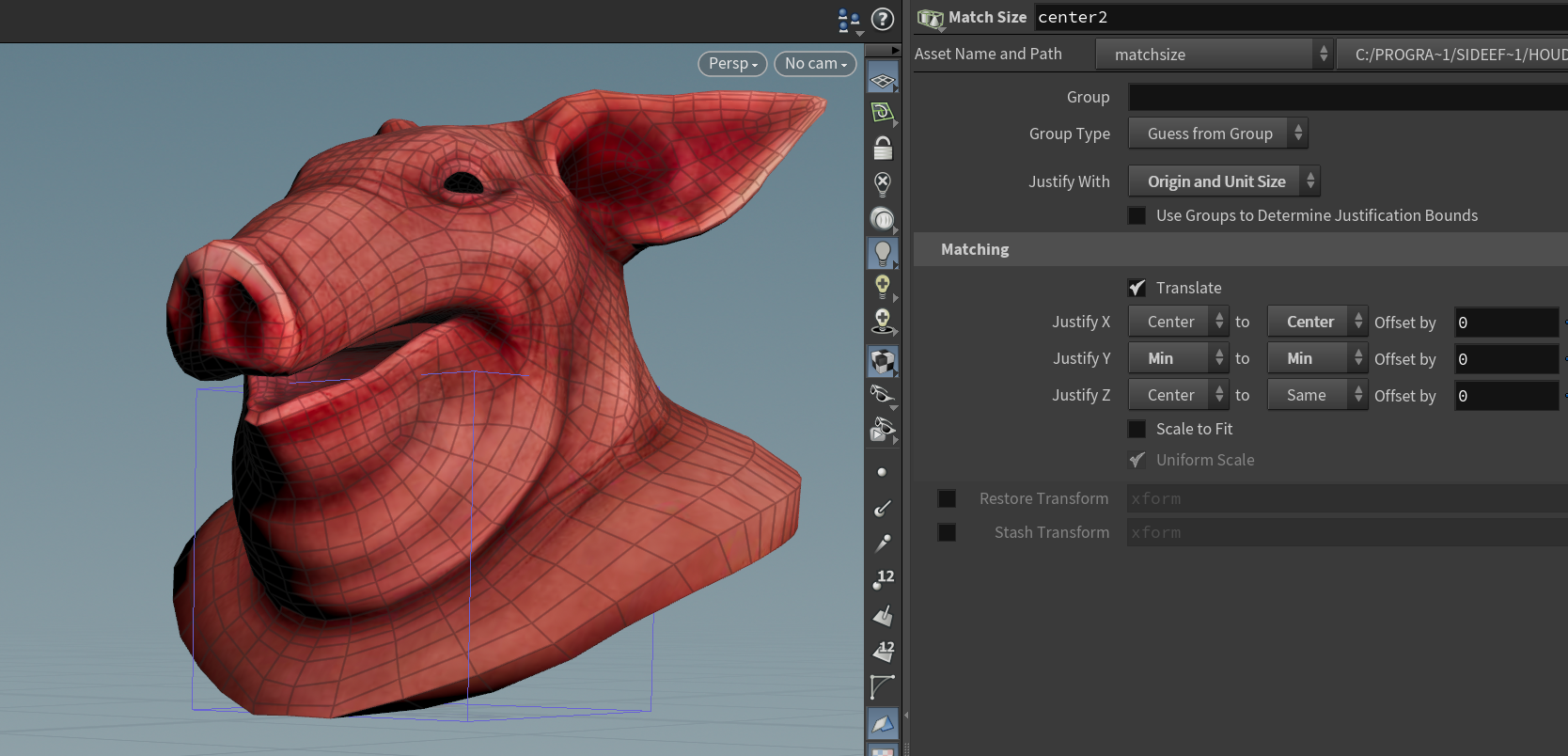
Match Size
The easiest way is using a Match Size node with “Justify Y” set to “Min”. It snaps the position only, and won’t affect the rotation.
Dihedral
To affect the rotation too, swalsch suggested using dihedral(). You can use it to rotate the normal towards a down vector.
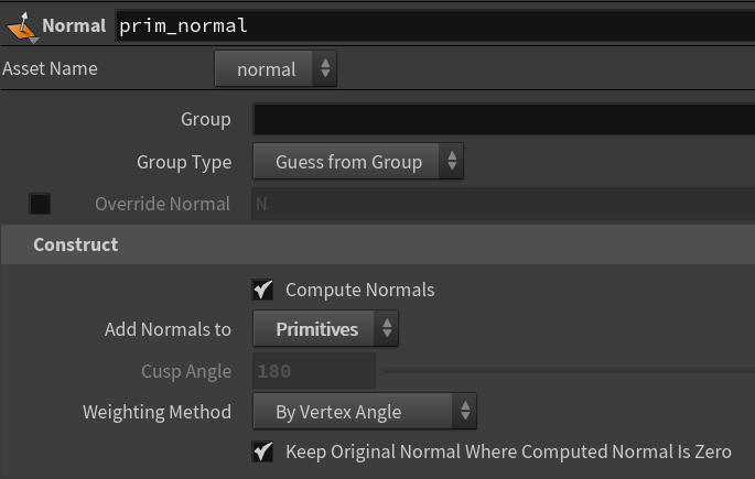
First the object needs prim normals, which you can add with a Normal node set to “Primitives”.
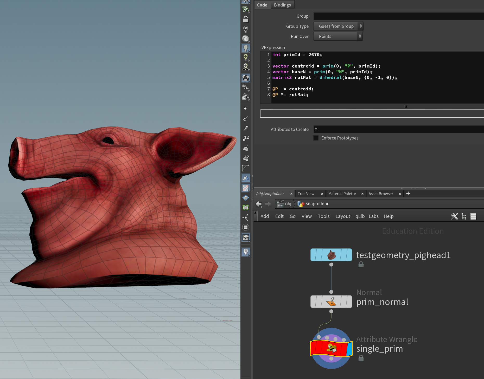
Next pick a prim to snap to the floor, get its normal and use dihedral() to build the rotation matrix.
int primIndex = 2670;

// Snap object to prim center
vector centroid = prim(0, "P", primIndex);
vector baseN = prim(0, "N", primIndex);
@P -= centroid;

// Rotate normal vector towards down vector
matrix3 rotMat = dihedral(baseN, {0, -1, 0});
@P *= rotMat;
To use multiple prims, make a prim group and average out the normals within that group.
// Get prims in a prim group called "bottom"
int prims[] = expandprimgroup(0, "bottom");
int primCount = len(prims);

// Find average position and normal
vector posSum = 0, normalSum = 0;
foreach (int primIndex; prims) {
    posSum += prim(0, "P", primIndex);
    normalSum += prim(0, "N", primIndex);
}

// Snap object to average position (same as getbbox_center(0, "bottom"))
v@P -= posSum / primCount;

// Rotate average normal towards down vector
matrix3 rotMat = dihedral(normalSum / primCount, {0, -1, 0});
v@P *= rotMat;
Extract Transform
The hackiest way is abusing Extract Transform. You flatten the prims to the floor, then approximate the transform for it.
This affects position and rotation, but isn’t as good as dihedral() since it won’t flip the object past 180 degrees.
- Blast all the prims except the ones you want to snap. Use a Transform node to center them and scale them to 0 on the Y axis.
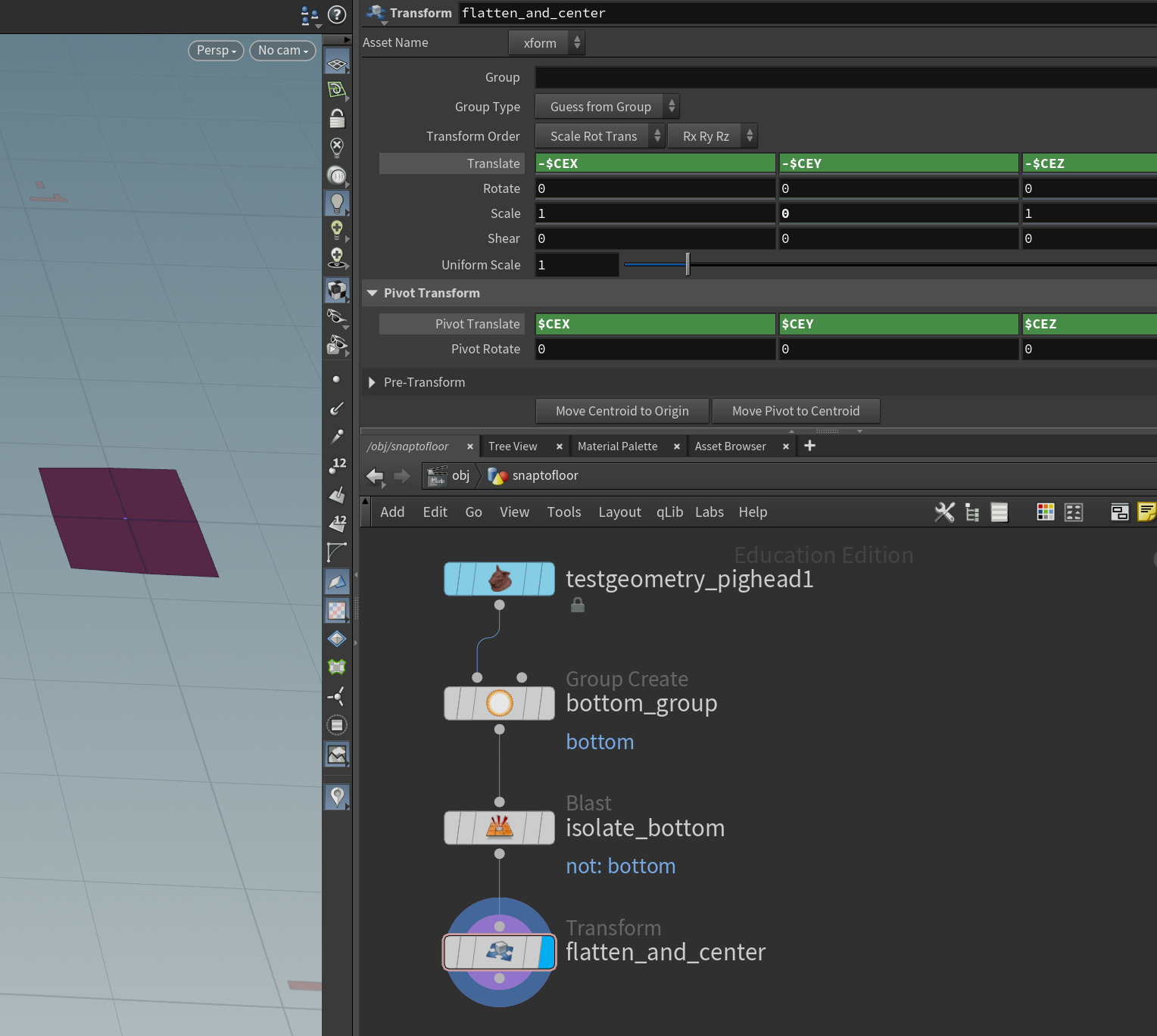
- Use Extract Transform to find the transform. Make sure “Extraction Method” is “Translation and Rotation” to avoid scaling and skewing!
- Use Transform Pieces to apply the transform, forcing the prims to the floor as much as possible.
![]()
FEM: Using real world physical units
Unlike the RBD Solver, the FEM Solver doesn’t list real world physical units. How do you use measurements with it?
I emailed SideFX, and they responded with some useful information:
I am told both Shape Stiffness and Volume Stiffness have units of Pascal when the stiffness multiplier is set to 1.
With the default Stiffness Multiplier of 1000, both these parameters would be in KPa.These coefficients have the following meaning:
shape_stiffness = 2x Lamé's second parameter
volume_stiffness = Lamé's first parameter
Conversion from other physical parameters, which are more commonly available:
If you have the Young’s modulus and the Poisson ratio of your material, you can compute the corresponding shape stiffness and volume stiffness parameters by:
shape_stiffness = youngs_modulus / ( 1 + poisson_ratio )
volume_stiffness = shape_stiffness * ( poisson_ratio / ( 1 - ( 2 * poisson_ratio ) ) )
The damping ratio parameters are unitless and should be chosen in between 0 and 1.
The attributes solidshapestiffness, solidvolumestiffness, etc. work as multipliers for the parameters that you specify on the object.
You could keep these between 0 and 1 if you like to dial in the relative stiffness for parts of the material, where the overall stiffness is determined by the shape stiffness and volume stiffness parameters.
Vellum: Stop wobbling, be rigid and bouncy
Vellum is usually wobbly like jelly, making hard objects tricky to achieve without an RBD Solver.
If you absolutely need Vellum, a great technique comes from Matt Estela.
- Go to the “Advanced” tab of the Vellum Solver and disable “Max Acceleration”.
- For any shapes you want to make rigid, add a “Shape Match” constraint and make it super stiff.
- Disable anything to do with smoothing or softening and lower the thickness.
Keep the topology as basic as possible and try increasing the substeps to make Shape Match even more stiff.
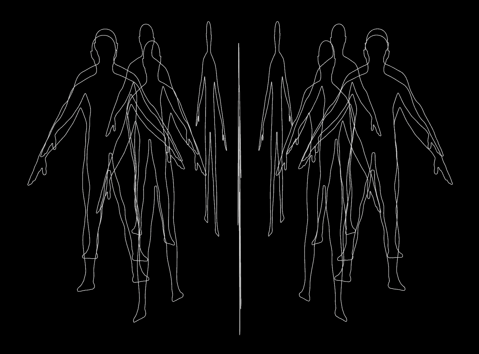
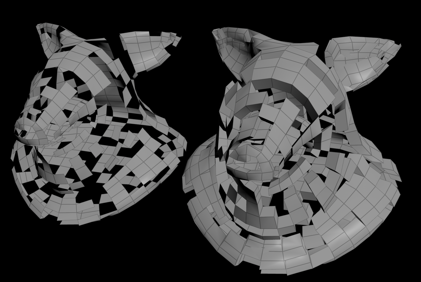
Stabilize and unstabilize geometry
Otherwise known as swapping reference frames, rest to animated, world to local, frozen to unfrozen…
Perhaps the best trick in Houdini is moving geometry to a rest pose, doing something and moving it back to an animated pose.
It fixes tons of issues like broken collisions, VDBs jumping around, plus aliasing and quantization artifacts.
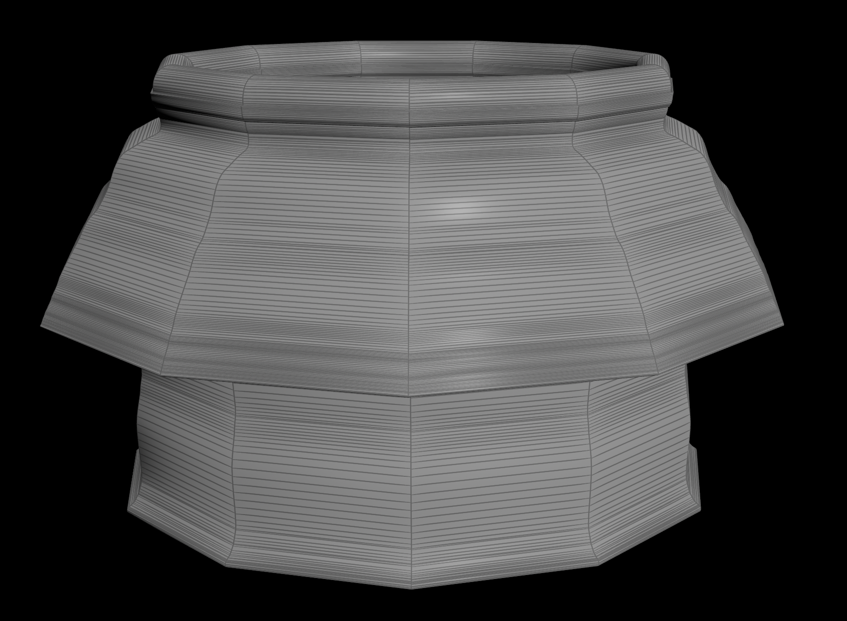
Rigid geometry
Extract Transform and Transform Pieces are your best friends.
- Use Time Shift to freeze the animated geometry. This is your rest pose.
- If possible, blast everything except a single prim for optimization.
- Use Extract Transform to calculate the transform from the animated prim to the frozen prim.
- Use Transform Pieces to stabilize the geometry. Make sure to tick “Invert Transformation”!
- Do stuff while it’s stabilized.
- Use Transform Pieces to move the geometry back to the animated pose.
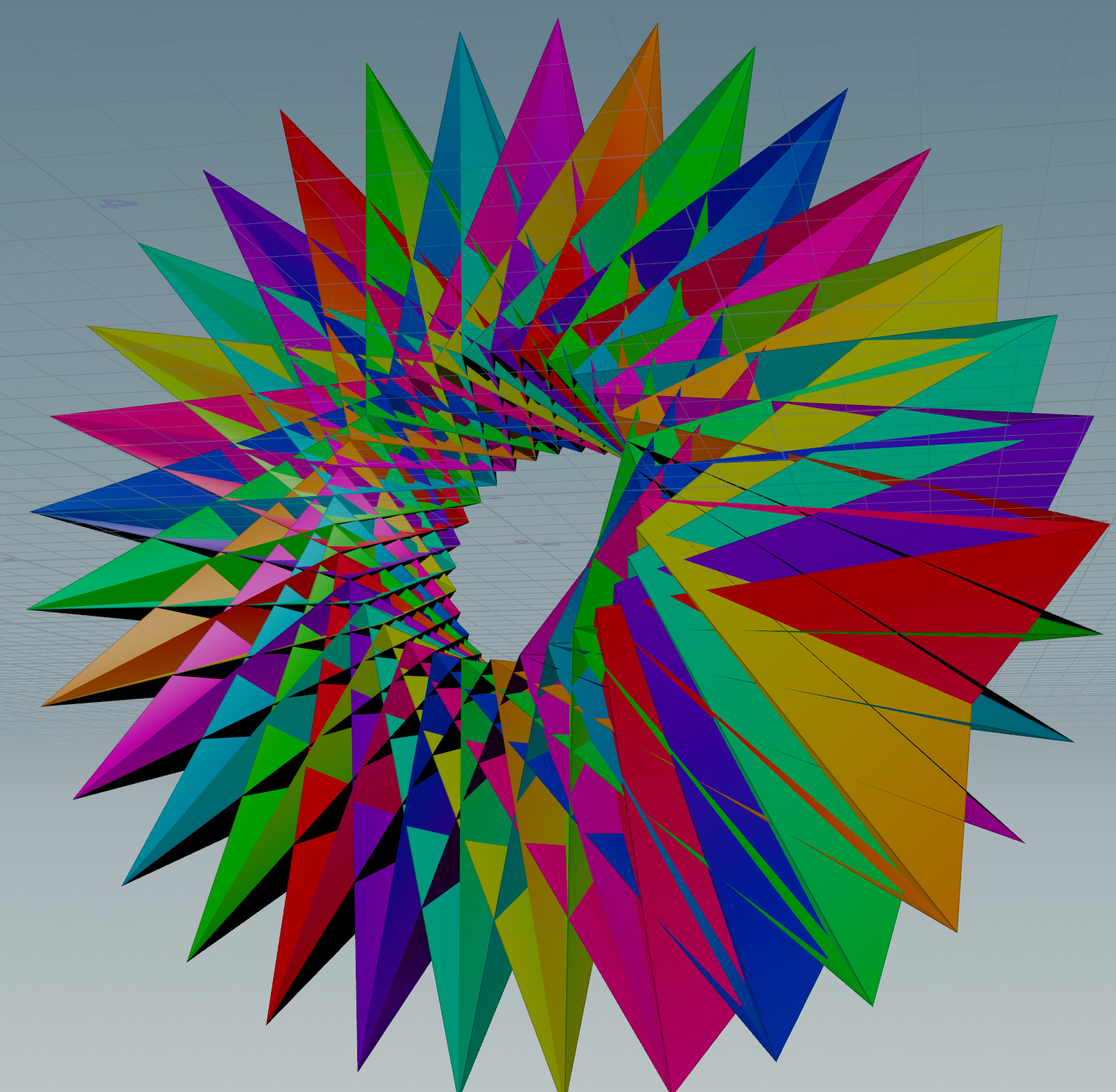
As well as Transform Pieces, you can set Extract Transform to output a matrix and transform manually in VEX:
// Extract Transform matrix from input 1
matrix mat = point(1, "transform", 0);
// Forward transform
v@P *= mat;
// Inverse transform
v@P *= invert(mat);
![]()
| Download the HIP file! | | — |
![]()
| Download the HIP file! | | — |
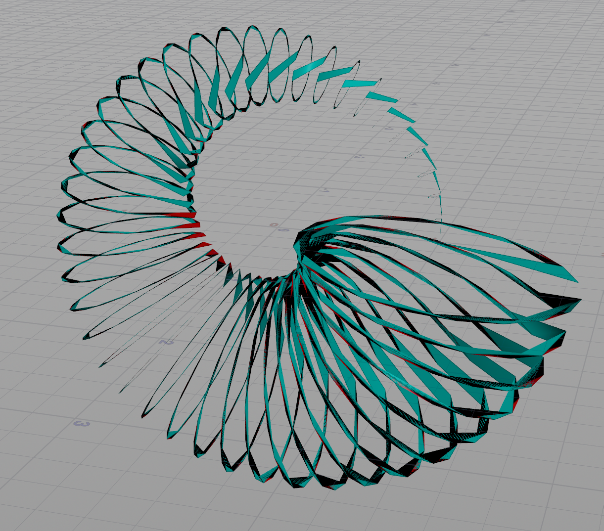
Bendy geometry
For simple cases, Point Deform is your best friend.
- Use Time Shift to freeze the animated geometry. This is your rest pose.
- Point Deform the animated geometry with the inputs in the wrong order, so it deforms from animated to rest.
- Do stuff while it’s frozen.
- Point Deform back with the inputs in the right order, so it deforms from rest to animated.
If you need better interpolation, try primuv() or Attribute Interpolate. This works great for proxy geometry, for example remeshed cloth.
- Use
xyzdist()to map the positions of the good geometry onto the proxy geometry, both in rest position.
xyzdist(1, v@P, i@near_prim, v@near_uv);
- Simulate the proxy geometry.
- In another wrangle, use
primuv()to match the good geometry’s position to the animated proxy.
v@P = primuv(1, "P", i@near_prim, v@near_uv);
Other ways to parent stuff
- Rivet is good for parenting objects to points. It only exists in the object context.
- Copy to Points is good since it applies
@orient,@Nand@upattributes. - PolyHinge is good for parenting to edges, though no one really uses it.
Primuv vs actual UVs
A common misconception is primuv() uses the actual UV map of the geometry. This would cause problems if the UVs overlapped.
Instead it uses intrinsic UVs. Intrinsic UVs are indexed by prim and range from 0 to 1 per prim. Since each prim is separated by index, it’ll never overlap.
| Regular UVs | Intrinsic UVS |
|---|---|
 |
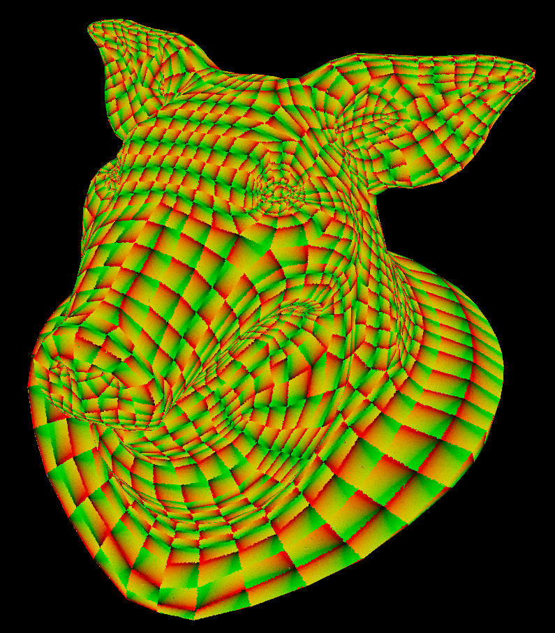 |
If you want to use the actual UVs, use uvsample() instead.
Fluids: Fix gap between surfaces
Usually liquids resting on a surface have a small gap due to the collision geometry, easier to see once rendered.
A tip from Raphael Gadot is to transfer normals from the surface onto the liquid with some falloff. This greatly improves the blending.
Optimize everything
Is your scene slow? Don’t blame Houdini, it’s likely you haven’t optimized properly.
- Using subdivided geometry? PolyReduce and Remesh it down to the simplest form.
- Using Copy to Points? Pack the geometry and use instancing. If not possible, make a few variants in a for loop and use packed versions of those.
- Using Vellum? Keep the overall substeps at 5-10 and focus on the relevant substeps, like collision substeps or constraint substeps.
- Using Alembic or USD? Freeze non-animated geometry with a Time Shift node so it never gets cached twice.
- Using surface collisions? Use Convex Hull, Convex Decomposition, PolyReduce and Remesh to simplify detailed geometry and improve collisions.
- Using volume collisions? Split animated and non-animated geometry into separate volumes, freeze the non-animated one with Time Shift, then merge with VDB Combine.
- Using Pyro? Keep the total voxel count as low as possible, a million is usually plenty. Convert to VDB to prune blank voxels from memory.
- Use File Caches religiously, and be sure to save your caches on a fast SSD instead of a HDD!
Use Houdini’s performance monitor to track down what’s slowest.
Be careful with velocity
Velocity is easy to overlook and hard to get right. I’ve rendered full shots before realising I forgot to put velocity on deforming geo, transfer it to packed geo, or it doesn’t line up.
A great tip from Lewis Taylor is to double check velocities from POP sims. It sometimes ignores POP forces and calculates an incorrect result.
For checking velocities, a tip from Ben Anderson is Time Shift a frame backward, template it and display velocity. You should see a line between the past and present position.
Be careful combining VDBs
Combining multiple pairs of VDBs is often unpredictable, for example combining two sims by density may skip velocity.
Make sure to combine each VDB pair separately, then feed all pairs into a merge node.
Be careful with typecasting
I used to do this to generate random velocities between -0.5 and 0.5. See if you can spot the problem.
v@v = rand(i@ptnum) - 0.5;
The issue is VEX uses the float version of rand(), making the result 1D:
float x = rand(i@ptnum);
v@v = x - 0.5;

To get a 3D result, there are two options. Either explicitly declare 0.5 as a vector:
v@v = rand(i@ptnum) - vector(0.5);
Or explicity declare rand() as a vector:
vector x = rand(i@ptnum);
v@v = x - 0.5;
This happens a lot, so always explicitly declare types to be safe!
Be careful with random
Even with fixed typecasting, there’s still a problem. See if you can spot it:
v@v = rand(i@ptnum) - vector(0.5);
What shape would you expect to see? Surely a sphere, since it’s centered at 0 and random in all directions?
Unfortunately it’s a cube, since the range is -0.5 to 0.5 on all axes separately.
Random direction, random length
To get a sphere and random vector lengths, use sample_sphere_uniform():
v@v = sample_sphere_uniform(rand(i@ptnum));
Roughly equivalent to the following:
v@v = normalize(rand(i@ptnum) - vector(0.5)) * rand(i@ptnum + 1);
Random direction, constant length
To get a sphere and normalized vector lengths, use sample_direction_uniform():
v@v = sample_direction_uniform(rand(i@ptnum));
Roughly equivalent to the following:
v@v = normalize(rand(i@ptnum) - vector(0.5));
Split vector magnitude and direction
Sometimes you need to change part of a vector but not the other, like to randomize velocity but inherit the magnitude. It’s easy with rotation, but here’s a more general approach:
// Deconstruction
vector dir = normalize(v@v);
float mag = length(v@v);

// Modify magnitude or direction here
dir = sample_direction_uniform(rand(@ptnum));

// Reconstruction, make sure direction is normalized
v@v = dir * mag;
POP: Make particles look like fluid
A key characteristic of fluid is how it sticks together, forming clumps and strands. POP Fluid tries to emulate this, but it doesn’t look as good as FLIP.
To get nicer clumps, a tip from Raphael Gadot is to use Attribute Blur set to “Proximity”. Though it won’t affect the motion, it looks incredible on still frames.
Smoke / Fluids: Fix moving colliders
Fluids often screw up whenever colliders move, like water in a moving cup or smoke in an elevator. Either the collider deletes the volume as it moves, or velocity doesn’t transfer properly from the collider.
A great fix comes from Raphael Gadot: Stabilise the collider, freeze it in place. Simulate in local space, apply forces in relative space, then invert back to world space. This works best for enclosed containers or pinned geometry, since it’s hard to mix local and world sims.
1. Relative gravity
- Add an
@upvector in world space (before Transform Pieces).
v@up = {0, 1, 0};
- Add a Gravity Force node to your sim (after Transform Pieces). Use the transformed
@upvector as your gravity force.
Force X = -9.81 * point(-1, 0, "up", 0)
Force Y = -9.81 * point(-1, 0, "up", 1)
Force Z = -9.81 * point(-1, 0, "up", 2)
Make sure the force is “Set Always”!
2. Relative acceleration
-
Add a Trail node set to “Calculate Velocity”, then enable “Calculate Acceleration”. It’s faster to do this after packing so it only trails one point.
-
Add another Gravity Force node, using negative
@accelas your force vector.
Force X = -point(-1, 0, "accel", 0)
Force Y = -point(-1, 0, "accel", 1)
Force Z = -point(-1, 0, "accel", 2)
Make sure the force is “Set Always”!
3. Stabilise (world to local)
- Pick a face on the collider you want to stabilise. Blast everything except that face.
- Time freeze that face with a Time Shift node.
- Use an Extract Transform node to compare the frozen face to the moving face. That tells you how the collider moves over time, allowing you to cancel out the movement.
- Pack everything else. Make sure to enable “No Point Velocities”.
- Plug the Pack into a Transform Pieces node, then plug Extract Transform into the other input.
- You should see the collider frozen in place. If not, try swapping the Time Shift to the other input in your Extract Transform node.
- Unpack and do your sim in local space.
- Pack the sim result.
- Add another Transform Pieces node with the same Extract Transform input. This time, set it to “Invert Transformation” to go back to world space.
- Unpack the world space result.
If you want to deal with open containers, the easiest way is to do a separate sim when the fluid exits the container. This is done by killing points outside the container, then feeding the killed points into the other sim. Make sure to nuke all point attributes to keep it clean for the next sim.
Another tip is use “Central Difference” when calculating the velocity. This gives the fluid more time to move away from the collider.
Cloth: Fix missing preroll
Cloth sims work best with preroll starting in a neutral rest pose. For example, the character starts in an A-pose or T-pose before transitioning into the animation. If anim screwed you over, never fear! Preroll can be added in Houdini.
With FBX
- Export the animated character as FBX. Make sure to include the skeleton!
- Import the character with a FBX Character Import node.
- Use a Skeleton Blend node to blend from the rest skeleton to the animated skeleton. If the rest skeleton has a bad pose, fix it with the Rig Pose node. Alternatively, export another FBX posed to your liking. FBX Character Import that animated skeleton as the rest skeleton.
- Use the Time Shift node to move the animation forward so it doesn’t bleed into the preroll. This can also be done in the “Timing” menu of FBX Character Import.
- Use Bone Deform to animate the skin based on Skeleton Blend.
![]()
| Download the HIP file! | | — |
Without FBX
Try using my node Fast Straight Skeleton 3D! It gives you rest and deforming skeletons you can use with Joint Capture Biharmonic.
To blend from T-Pose to animated, plug the animation into the first input and the T-Pose into the second input. Then blend the two skeletons with Skeleton Blend.
Afterwards you can use Joint Capture Biharmonic to deform the skin using Bone Deform. Make sure the centroid method is “Center of Mass” for best results!
Cloth: Fix rest pose clipping
Cloth sims screw up from clipping, especially when clipped from the start. One option is growing the character into the cloth.
- Disable gravity in the cloth sim.
- Use Smooth, Peak or VDB Reshape to shrink the character.
- Animate the character growing.
- Enable gravity in the cloth sim.
- Use the Time Shift node to move the animation forward so it doesn’t bleed into the growing.
Cloth: Layer stacking
One little known feature of Vellum Cloth (at least to me) is layering. It can improve the physics of overlapping garments, like jackets on top of t-shirts.
- In Vellum Configure Cloth, use the “Layer” setting to define the ordering, bottom to top.
- On the Vellum Solver under “Collisions”, enable “Layer Shock”. Lower layers are simulated much heavier than higher layers.
Karma: Fix motion blur
Motion blur in Karma can be pretty unpredictable, especially with packed instances.
A great fix comes from Matt Estela: just add a Cache node set to “Rolling Window”. Usually I use 1 frame before and 1 frame after.
This is faster than the new Motion Blur node, which caches the entire timeline at once. It also fixes issues with animated materials.
Attribute min / max / average…
Use Attribute Promote set to “Detail” with the appropriate mode.
Alternating rows for brick walls
The tricky part about modelling brick walls is the alternating pattern. Every second row is slid across by half a brick’s width. How would you create this pattern? Manual interpolation? Primuv?
An easy way is working subtractively. Take the base curve and resample it. This gives you the first row. For the second row, subdivide the first. Use a “Group by Range” node to select every second point, then delete them with a “Dissolve” node.
Access context geometry inside solver
If you need geometry in a context that doesn’t provide it (like the forces of a Vellum Solver), just drop down a SOP Solver. You can use Object Merge inside a SOP Solver to grab geometry from anywhere else too. Great for feedback loops!
Pyro: Fix mushrooms
Many techniques work depending on the situation. Sometimes more randomisation is needed, other times the velocity needs reducing.
A common technique is cranking up the disturbance. Controlling it by speed helps add it where mushrooms are likely to form.
This groups the points where cycles occur. To repair the cycles, you can cut or remove these points with PolyCut.
Negative frame ranges
Seems obvious but worth noting: Unlike some software, Houdini supports negative frame ranges.
For preroll you can always start simulating on a negative frame without needing to time shift anything.
Fluids: Fix density loss
Don’t take this section seriously. These are just techniques which seem to work for me.
Density loss often happens when Surface Tension is enabled. Droplets tend to disappear when bunched too close together, so try disabling it before anything else.
Grid Scale and Particle Radius Scale also affect the density. According to SideFX, if the Particle Radius Scale divided by the Grid Scale is at least sqrt(3)/2, it will never be underresolved.
No idea if this affects density, but just in case here’s the minimum:
Particle Radius Scale = Grid Scale × (sqrt(3)/2)
Grid Scale = Particle Radius Scale / (sqrt(3)/2)